7 Generalized Linear Models
In the preceding chapters we got acquainted with the linear model as an extremely flexible tool to represent dependencies between predictors and outcome variables. We saw how factors and covariates gracefully work together and how complex research designs can be captured by multi-level random effects. It was all about specifying an appropriate (and often sophisticated) right-hand side of the regression formula, the predictor term. In contrast, little space has been dedicated to the outcome variables, except that sometimes we used log-transformed outcomes to accommodate the Gaussian error term. That is now going to change, and we will start by examining the assumptions that are associated with the outcome variable.
A particular question is probably lurking in the minds of readers with classic statistics training: What happened to the process of checking assumptions on ANOVA (and alike) and where are all the neat tests that supposedly check for Normality, constant variance and such? The Gaussian linear model, which we used throughout 4 and 6, shares these assumptions, the three crucial assumptions being:
- Linearity of the association between predictors and outcome variable.
- Gaussian distribution of responses
- constant variance of response distribution
In the next section we will review these assumptions and lead them ad absurdum. Simply put, with real world outcome measures there is no such thing as Gaussian distribution and true linearity. Checking assumptions on a model that you know is inappropriate, seems a futile exercise, unless better alternatives are available, and that is the case: with Generalized Linear Models (GLMs) we extend our regression modeling framework once again, this time focusing on the outcome variables and their shape of randomness.
As we will see, GLMs solves some common problems with linearity and gives us more choices on the shape of randomness. To say that once and for all: What GLMs do not do is relax the assumptions of linear models. And because I have met at least one seasoned researcher who divided the world of data into two categories, “parametric data,” that meets ANOVA assumptions, and “non-parametric data” that does not, let me get this perfectly straight: data is neither parametric nor non-parametric. Instead, data is the result of a process that distributes measures in some form and a good model aligns to this form. Second, a model is parametric, when the statistics it produces have a useful interpretations, like the intercept is the group mean of the reference group and the intercept random effect represents the variation between individuals. All models presented in this chapter (and this book) fulfill this requirement and all are parametric. There may be just one counter-example, which is polynomial regression 5.5, which we used for its ability to render non-monotonic curves. The polynomial coefficients have no interpretation in terms of the cognitive processes leading to the Uncanny Valley. However, as we have seen in 5.5.1, they can easily be used to derive meaningful parameters, such as the positions of shoulder and trough. A clear example of a non-parametric method is the Mann-Withney U-test, which compares the sums of ranks between groups, which typically has no useful interpretation.
The GLM framework rests on two extensions that bring us a huge step closer to our precious data. The first one is the link function a mathematical trick that establishes linearity in many situations. The second is to select a shape of randomness that matches the type of outcome variable, and removes the difficult assumption of constant variance. After we established the elements of the GLM framework 7.1, I will introduce a good dozen of model families, that leaves little reason to ever fall back to the Gaussian distributions and data transformations, let alone unintelligible non-parametric procedures. As we will see, there almost always is a clear choice right at the beginning that largely depends on the properties of the response variable, for example:
- Poisson LM is the first choice for outcome variables that are counted (with no upper limit), like number of errors.
- Binomial (aka logistic) LM covers the case of successful task completion, where counts have an upper boundary.
These two GLM families have been around for more many decades in statistical practice, and they just found a new home under the GLM umbrella. For some other types of outcome variables good default models have been lacking, such as rating scale responses and time-on-task and reaction times. Luckily, with recent developments in Bayesian regression engines the choice of random distributions has become much broader and now also covers distribution families that are suited for these very common types of measures. For RT and ToT, I will suggest exponentially-modified Gaussian (ExGauss) models or, to some extent, Gamma models. For rating scales, where responses fall into a few ordered categories, ordinal logistic regression is a generally accepted approach, but for (quasi)continuous rating scales I will introduce a rather novel approach, Beta regression.
Too many choices can be a burden, but as we will see, most of the time the appropriate model family is obvious. For the impatient readers, here is the recipe: Answer the following three questions about the outcome variable and follow (Figure 7.1).
- Is the outcome variable discrete or continuous?
- What are the lower and upper boundaries of outcome measures?
- Can we expect over-dispersion?
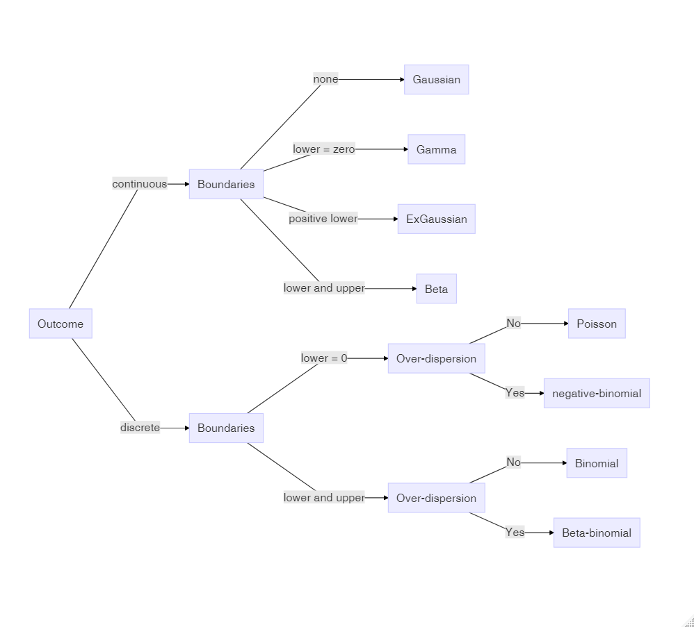
Figure 7.1: Decision chart for Generalized Linear Models
To make it even easier, it is practically always adequate and safe to answer Yes to the third question (over-dispersion). Based on these questions, the graph below identifies the correct distribution family and you can jump right to respective section, if you need a quick answer. In the following section (7.1)), I will provide a general explanation of why GLMs are needed and how they are constructed by choosing a response distribution (7.1.2) and a link function (7.1.1). The remainder of the chapter is organized by types of measures that are typical for design research: count data (7.2), duration measures (7.3)) and rating scales (7.4). Together with chapter 6, this introduces the family of models called Generalized Multi-level Linear Models (GMLM), which covers a huge variety of research situations. The chapter closes with a brief introduction to an even mightier class of models: GMLMs still have certain limitations. One of them is that they are all about estimating average performance. Distributional models are one further step of abstraction and they apply when the research is concerned with variance, actually (7.5).
7.1 Elements of Generalized Linear Models
GLM is a framework for modelling that produces a family of models (Figure 7.1). Every member of this family uses a specific link functions to establish linearity and a particular distribution, that has an adequate shape and mean-variance relationship.
Sometimes GLMs are mistaken as a way to relax assumptions of linear models, (or even called non-parametric). They are definitely not! Every member makes precise assumptions on the level of measurement and the shape of randomness. One can even argue that Poisson, Binomial and exponential regression are stricter than Gaussian, as they use only one parameter, with the consequence of a tight association between variance and mean. A few members of GLM are classic: Poisson, Binomial (aka logistic) and exponential regression have routinely been used before they were united under the hood of GLM. These and a few others are called canonical GLMs, as they possess some convenient mathematical properties, that made efficient estimation possible, back in the days of limited computing power.
For a first understanding of Generalized Linear Models, you should know that linear models are one family of Generalized Linear Models, which we call a Gaussian linear model. The three crucial assumptions of Gaussian linear models are encoded in the model formula:
\[ \begin{aligned} \mu_i &=\beta_0+ \beta_1 x_{1i}+ \dots +\beta_k x_{ki}\\ y_i &\sim \textrm{Gaus}(\mu_i,\sigma) \end{aligned} \]
The first term, we call the structural part and it represents the systematic quantitative relations we expect to find in the data. When it is a sum of products, like above, we call it linear. Linearity is a frequently under-regarded assumption of linear models and it is doomed to fail 7.1.1. The second term defines the pattern of randomness and it hosts two further assumptions: Gaussian distribution and constant error variance of the random component. The latter might not seem obvious, but is given by the fact that there is just a single value for the standard error \(\sigma\).
In classic statistics education, the tendency is still to present these assumptions as preconditions for a successful ANOVA or linear regression. The very term precondition suggest, that they need to be checked upfront and the classic statisticians are used to deploy a zoo of null hypothesis tests for this purpose, although it is widely held among statisticians that this practice is illogical. If an assumptions seems to be violated, let’s say Normality, researchers then often turn to non-parametric tests. Many also just continue with ANOVA and add some shameful statements to the discussion of results or humbly cite one research paper that claims ANOVAs robustness to this or that violation.
The parameters of a polynomial model usually don’t have a direct interpretation. However, we saw that useful parameters, such as the minimum of the curve, can be derived. Therefore, polynomial models are sometimes called semiparametric. As an example for a non-parametric test, the Mann-Whitney U statistic is composed of the number of times observations in group A are larger than in group B. The resulting sum U usually bears little relation to any real world process or question. Strictly speaking, the label non-parametric has nothing to do with ANOVA assumptions. It refers to the usefulness of parameters. A research problem, where U as the sum of wins has a useful interpretation could be that in some dueling disciplines, such as Fencing, team competitions are constructed by letting every athlete from a team duel every member of the opponent team. Only under such circumstances would we call the U-test parametric.
7.1.1 Re-linking linearity
Linearity means that we increase the predictor by a fixed unit, the outcome will follow suit by a constant amount. In the chapter on Linear Models 4, we encountered several situations where linearity was violated.
- In 4.3.5 increasing amount of training by one session did result in rather different amount of learning. In effect, we used not an LRM, but ordered factors to estimate the learning curves.
- In 5.4.3, two pills did not reduce headache by the sum of each pill alone. We used conditional effects when two or more interventions improve the same process in a non-linear way.
- and in 5.5 we used polynomials to estimate wildly curved relationships
The case of Polynomial regression is special in two ways: first, the curvature itself is of theoretical interest (e.g. finding the “trough” of the Uncanny Valley effect). Second, a polynomial curve (of second degree or more) is no longer monotonously increasing (or decreasing). In contrast, learning curves and saturation effects have in common that in both situations outcome steadily increases (or decreases) when we add more to the predictor side. There just is a limit to performance, which is reached asymptotically (which means the curve never really flattens).
For the learning process in the IPump study we earlier used an OFM with stairways coding to account for this non-linearity (@ref(#ofm)), but that has one disadvantage. From a practical perspective it would interesting to know, how performance improves when practice continues. What would be performance in (hypothetical) sessions 4, 5 and 10. Because the OFM just makes up one estimate for every level, there is no way to get predictions beyond the observed range.
With an LRM, the slope parameter applies to all steps, which gives us the possibility of deriving predictions beyond the observed range. To demonstrate this on the deviations from optimal path, the following code estimates a plain LRM and then injects some new (virtual) data to get extrapolations beyond the observed three tasks. Note that the virtual data comes without a response variable, as this is what the model provides (Table 7.1).
attach(IPump)M_LRM_1 <- stan_glm(deviations ~ 1 + session,
data = D_Novel
)D_extra <-
tibble(
session = as.integer(c(0:9)),
range = if_else(session < 3,
"observed", "extrapolated"
)
) %>%
as_tbl_obs()
D_extra | Obs | session | range |
|---|---|---|
| 1 | 0 | observed |
| 2 | 1 | observed |
| 3 | 2 | observed |
| 4 | 3 | extrapolated |
| 5 | 4 | extrapolated |
| 6 | 5 | extrapolated |
| 7 | 6 | extrapolated |
| 8 | 7 | extrapolated |
| 9 | 8 | extrapolated |
| 10 | 9 | extrapolated |
predict(M_LRM_1,
  newdata = D_extra
) %>%
  left_join(D_extra) %>%
  ggplot(aes(
    x = session, y = center,
    ymin = lower, ymax = upper,
    color = range
  )) +
  geom_step() +
  geom_hline(aes(yintercept = 0, color = "impossible predictions below"), linetype = 2) +
  scale_x_continuous(breaks = 0:10) +
  ylim(-1, 1) +
  labs(y = "deviations", col = NULL)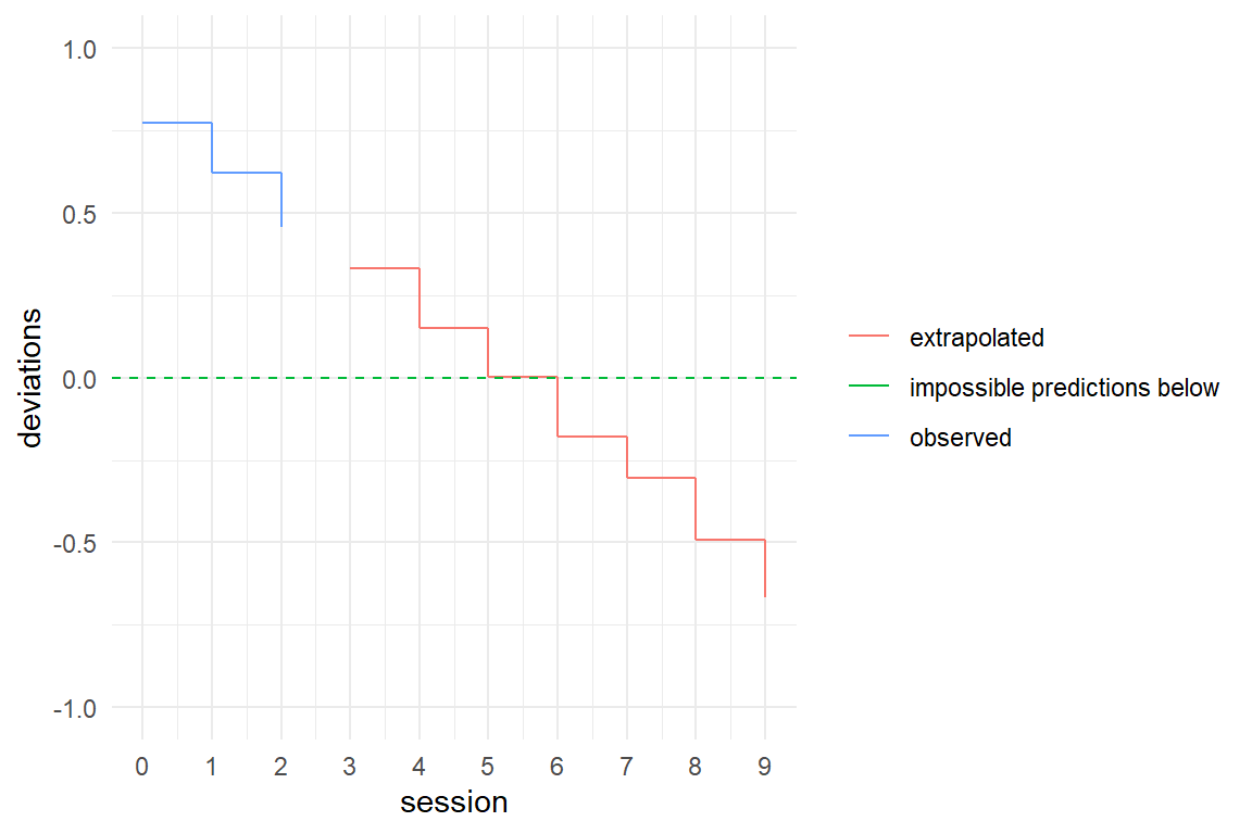
Figure 7.2: Trying to predict future performance by a linear model produces inpossible predictions
If we use a continuous linear model to predict future outcomes of a learning curve, negative values are eventually produced, which is impossible. Non-linearity is not just a problem with learning curves, but happens to all outcomes that have natural lower or upper boundaries. All known outcome variables in the universe have boundaries, just to mention velocity and temperature (on spacetime the jury is still out). It is an inescapable, that all our ephemeral measures in design research have boundaries and strictly cannot have linear associations:
- Errors and other countable incidences are bounded at zero
- Rating scales are bounded at the lower and upper extreme item
- Task completion has a lower bound of zero and the number of tasks as an upper bound.
- Temporal measures formally have lower bound of zero, but psychologically, the lower bound always is a positive number.
The strength of the linear term is its versatility in specifying multiple relations between predictor variables and outcome. It’s Achilles heel is that it assumes measures without boundaries. Generalized linear models use a simple mathematical trick that keeps a linear terms, but confines the fitted responses to the natural boundaries of the measures. In linear models, the linear term is mapped directly to fitted responses \(\mu_i\):
\[ \mu_i = \beta_0 + x_{1i}\beta_1 \]
In GLMs, an additional layer sits between the fitted response \(\mu\) and the linear term: The linear predictor \(\theta\) has the desired range of \([-\infty; \infty]\) and is linked directly to the linear term. In turn, we choose a link function \(\phi\) that up-scales the bounded range of measures (\(\mu\)). The inverse of the link function (\(\phi^{-1}\)) is called the mean function and it does the opposite by down-scaling the linear predictor to the range of measures.
\[ \begin{aligned} \theta_i &\in [-\infty; \infty]\\ \theta_i &= \beta_0 + x_{1i} \beta_1\\ \theta_i &= \phi( \mu_i)\\ \mu_i &= \phi^{-1}(\theta_i) \end{aligned} \] The question is: what mathematical function transforms a bounded space into an unbounded? A link function \(\phi\) must fulfill two criteria:
- mapping from the (linear) range \([-\infty; \infty]\) to the range of the response, e.g. \([0; \infty]\).
- be monotonically increasing, such that the order is preserved
A monotonically increasing function always preserves the order, such that the following holds for a link function.
\[ \theta_i > \theta_j \rightarrow \phi(\theta_i) > \phi(\theta_j) \rightarrow \mu_i > \mu_j \]
It would be devastating if a link function would not preserve order, but there is another useful side-effect of monotony: if a function \(\phi\) is monotonous, then there exists an inverse function \(\phi^{-1}\), which is called the mean function, as it transforms back to the fitted responses \(\mu_i\). For example, \(x^2\) is not monotonous and its inverse, \(\sqrt{x}\), produces two results (e.g. \(\sqrt{x} = [2, -2]\)) and therefore is not a even a function, strictly speaking.
A typical case is count variables with a lower boundary of zero and no upper bound. The logarithm is a function that maps positive numbers to the linear range \([-\infty; \infty]\), in the way that numbers smaller than One become negative.
log(c(2, 1, .5))## [1] 0.693 0.000 -0.693The logarithm has the exponential function as a counterpart, which bends the linear range back into the boundaries. Other measures, like success rates or rating scales, have lower and upper boundaries. A suitable pair of functions is the logit link function and the logistic mean function (Figure 7.3).
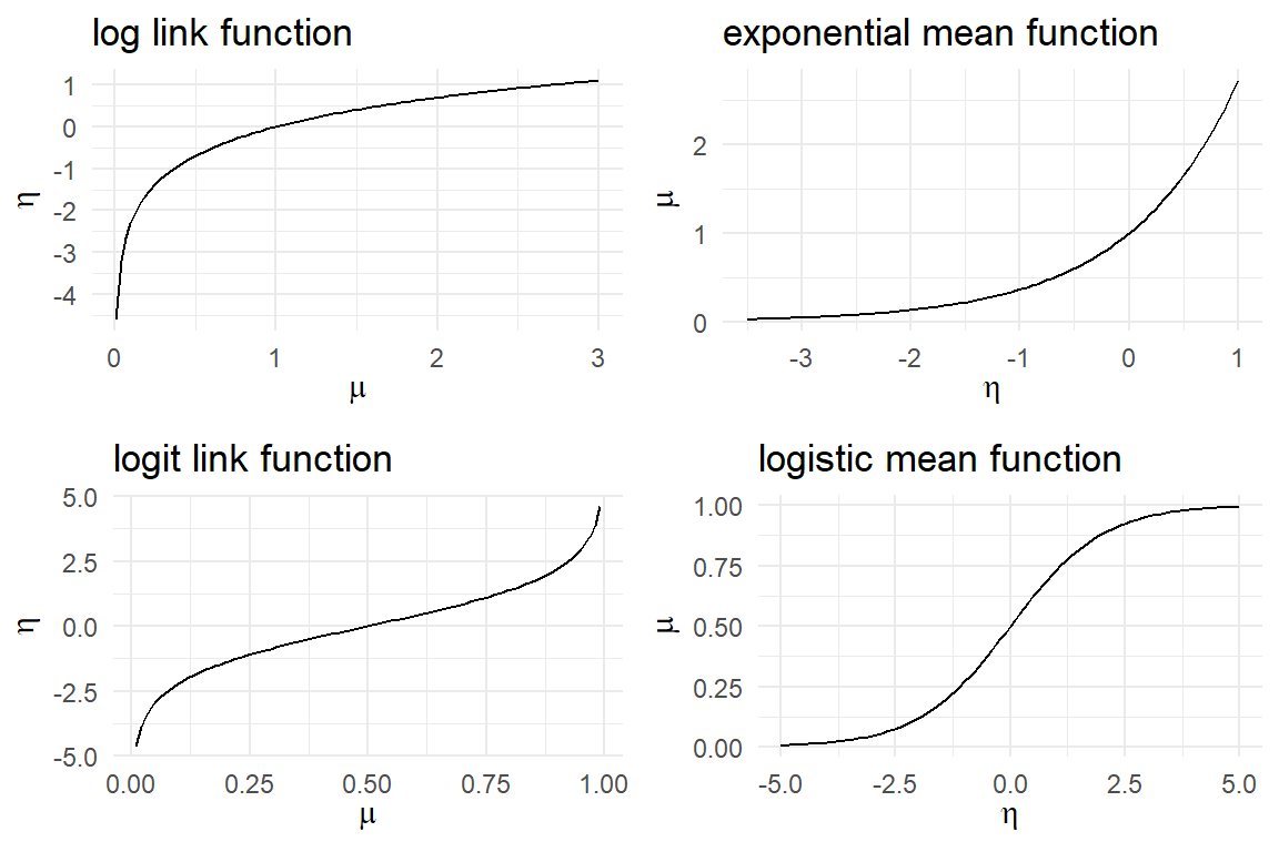
Figure 7.3: Log and logit link functions expand the bounded range of measures. Mean functions do the reverse.
Using the link function comes at a cost: the linear coefficients \(\beta_i\) is losing its interpretation as increment-per-unit and no longer has a natural interpretation. Later, we will see that logarithmic and logit scales gain an intuitive interpretation when parameters are exponentiated, \(\textrm{exp}(\beta_i)\) (@ref(speaking-multipliers and 7.2.2.3).
Who needs a well-defined link between observations and fitted responses? Applied design researchers do when predictions are their business. In the IPump study it is compelling to ask: “how will the nurse perform in session 4?” or “When will he reach error-free operation?” In 7.2.1.2 we will see a non-linear learning process becoming an almost straight line on the logarithmic scale.
7.1.2 Choosing patterns of randomness
The second term of a linear model, \(y_i \sim Norm(\mu_i, \sigma)\) states that the observed values are drawn from Gaussian distributions (3.5.2.6). But Gaussian distributions have the same problem as the linearity assumption: the range is \([-\infty; \infty]\).
The problem can be demonstrated by simulating observations, using a Gaussian pattern of randomness, and see how this fails to produce realistic data. Imagine a study comparing a novel and a legacy interface design for medical infusion pumps. The researchers let trained nurses perform a single task on both devices and count the errors. Assuming, the average number of errors per tasks is \(\mu_L = 3\) for the legacy device and \(\mu_N = 1.2\) for the novel device, with standard deviation of \(\sigma = .8\). We simulate data from a factorial linear model, ashown in Figure 7.4.
set.seed(84)
N <- 80
D_pumps_sim <-
  tibble(
    Design = rep(c("L", "N"), N / 2),
    mu = if_else(Design == "L", 3, 1.2),
    errors = rnorm(N, mu, sd = 1)
  ) %>%
  as_tbl_obs()
D_pumps_sim %>%
ggplot(aes(x = errors)) +
facet_grid(~Design) +
geom_histogram(bins = 20) +
geom_vline(aes(xintercept = 0)) +
coord_flip() +
labs(colour = "")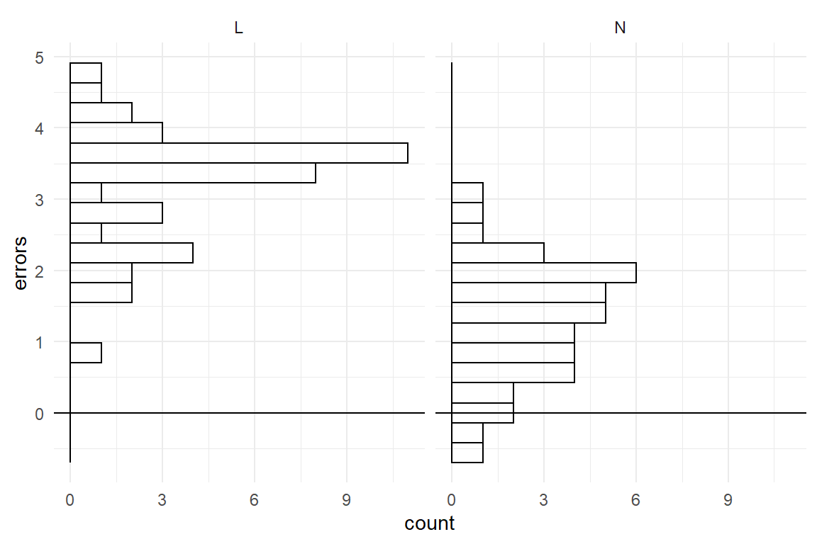
Figure 7.4: Simulation with Gaussian error terms produces impossible values.
We immediately see, that simulation with Gaussian distributions is inappropriate: a substantial number of simulated observations is negative, which strictly makes no sense for error counts. The pragmatic and impatient reader may suggest to adjust the standard deviation (or move the averages up) to make negative values less unlikely. That would be a poor solution as Gaussian distributions support the full range of real numbers, no matter how small the variance is (but not zero). There is always a chance of negative simulations, as tiny as it may be. Repeatedly running the simulation until pumps contains exclusively positive numbers (and zero), would compromise the idea of random numbers itself. We can simply conclude that any model that assumes normally distributed errors must be wrong when the outcome is bounded below or above, which means: always.
Recall how linearity is gradually bent when a magnitude approaches its natural limit. A similar effect occurs for distributions. Distributions that respect a lower or upper limit get squeezed like chewing gum into a corner when approaching the boundaries. Review the sections on Binomial 3.5.2.3 and Poisson distributions 3.5.2.4 for illustrations. As a matter of fact, a lot of real data in design research is skewed that way, making Gaussian distributions a poor fit. The only situation where Gaussian distributions are reasonable approximations is when the outcomes are far off the boundaries. An example of that is the approximation of Binomial outcomes (lower and upper bound), when the probability of success is around 50%. That is also the only point, where a Binomial distribution is truly symmetric.
In contrast, a common misconception is that the Gaussian distribution is a getting better at approximation, when sample sizes are large. This is simply wrong. What really happens, is that increasing the number of observations renders the true distribution more clearly.
In chapter 3.5.2 a number of random distributions were introduced, together with conditions of when they arise. The major criteria were related to properties of the outcome measure: how it is bounded and whether it is discrete (countable) or continuous. Generalized Linear Models give the researcher a larger choice for modeling the random component and Table 7.2 lists some common candidates.
| boundaries | discrete | continuous |
|---|---|---|
| unbounded | Normal | |
| lower | Poisson | Exponential |
| lower and upper | Binomial | Beta |
That is not to say that these five are the only possible choices. Many dozens of statistical distributions are known and these five are just making the least assumptions on the shape of randomness in their class (mathematicians call this maximum entropy distributions). In fact, we will soon discover that real data frequently violates principles of these distributions. For example, count measures in behavioral research typically show more error variance than is allowed by Poisson distributions. As we will see in 7.2.3, Poisson distribution can still be used in such cases with some additional tweaks borrowed from multi-level modeling (observation-level random effects).
Response times in design research are particularly “misbehaved,” as they do not have their lower boundary at zero, but at the lowest human possible time to solve the task. The complication arises that most continuous distributions have a lower boundary of exactly zero. In case of response times, we will take advantage of the fact, that modern Bayesian estimation engines support a larger range of distributions than ever seen before. The stan_glm regression engine has been designed with downwards compatibility in mind, which is why it does not include newer distributions. In contrast, the package brms is less hampered by legacy and gives many more choices, such as the Exponential-Gaussian distribution for ToT.
7.1.3 Mean-variance relationship
The third assumption of linear models is rooted in the random component term as well. Recall, that there is just one parameter \(\sigma\) for the dispersion of randomness and that any Gaussian distribution’s dispersion is exclusively determined by \(\sigma\). That is more of a problem as it may sound, at first. In most real data, the dispersion of randomness depends on the location, as can be illustrated by the following simulation.
Imagine a survey on commuter behavior that asks the following questions:
- How long is your daily route?
- How long does it typically take to go to work?
- What are the maximum and minimum travel times you remember?
If we simulate such data from a linear model, the relationship between length of route and travel time would look like a evenly wide band, which is due to the constant variance (Figure 7.5).
N <- 100
tibble(
  Obs = as.factor(1:N),
  km = runif(N, 2, 40),
  min = rnorm(N, km * 2, 10)
) %>%
  ggplot(aes(x = km, y = min)) +
  geom_point() +
  geom_quantile(quantiles = c(.25, .5, .75))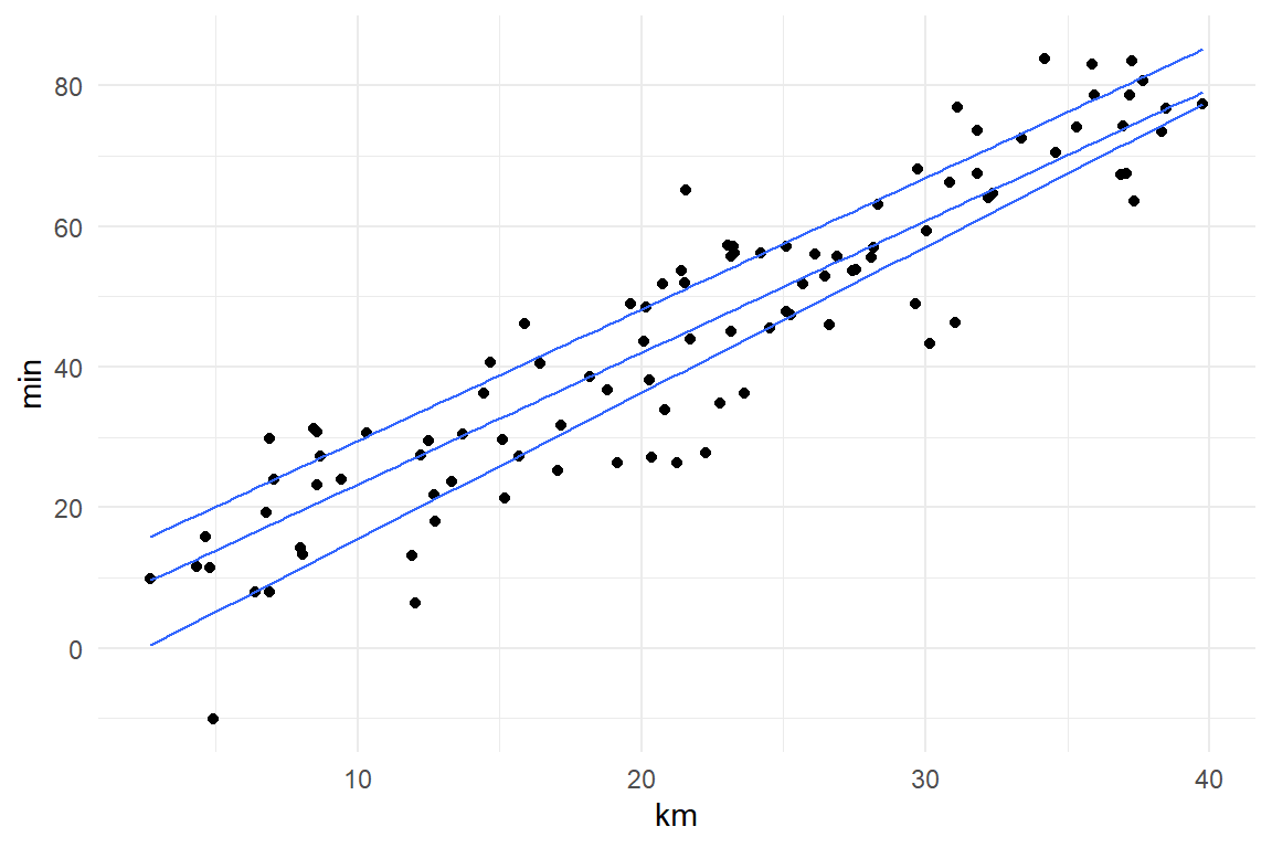
Figure 7.5: A Gaussian linear simulation of travel times (min) depending on distance (km) results in an unrealistic mean-variance relationship.
What is unrealistic is that persons who live right around the corner experience the same range of possible travel times than people who drive dozens of kilometers. That does not seem right.
Gaussian distributions are a special case, because most other distributions do not have constant variance. For example, a Gamma distribution takes two parameters, shape \(alpha\) and scale \(tau\) and both of them influence mean and variance of the distribution, such that the error variance increases by the square of the mean (Figure 7.6))
\[ \begin{aligned} Y &\sim \textrm{Gamma}(\alpha, \theta)\\ E(Y) &= \alpha \theta\\ \textrm{Var}(Y) &= \alpha \theta^2\\ \textrm{Var}(Y) &= E(Y) \theta \end{aligned} \]
tibble(
  km = runif(100, 2, 40),
  min = rgamma(100, shape = km * .5, scale = 4)
) %>%
  ggplot(aes(x = km, y = min)) +
  geom_point() +
  geom_quantile(quantiles = c(.25, .5, .75))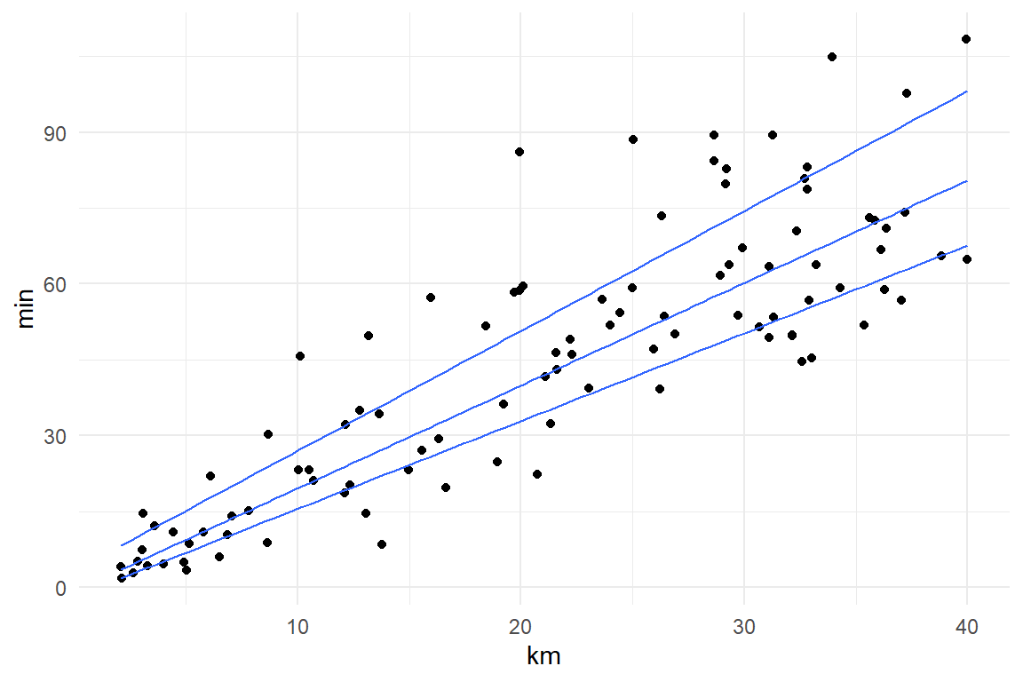
Figure 7.6: A Gamma simulation of travel times (min) depending on distance (km) results in a realistic mean-variance relationship.
A similar situation arises for count data. When counting user errors, we would expect a larger variance for complex tasks and interfaces, e.g. writing an article in a word processor, as compared to the rather simple situation like operating a medical infusion pump. For count data, the Poisson distribution is often a starting point and for Poisson distributed variables, mean and variance are both exactly determined by the Poisson rate parameter \(\lambda\), and therefore strictly connected to each other. Figure 7.7 shows hypothetical data from two tasks with very different error rates.
\[ \begin{aligned} Y &\sim \textrm{Poisson}(\lambda)\\ \textrm{Var}(Y) &= E(Y) = \lambda \end{aligned} \]
tibble(
  Task = rep(c("writing article", "using infusion pump"), 50),
  errors = rpois(100,
    lambda = if_else(Task == "writing article",
      200, 8
    )
  )
) %>%
  ggplot(aes(x = Task, y = errors)) +
  geom_boxplot() +
  geom_jitter()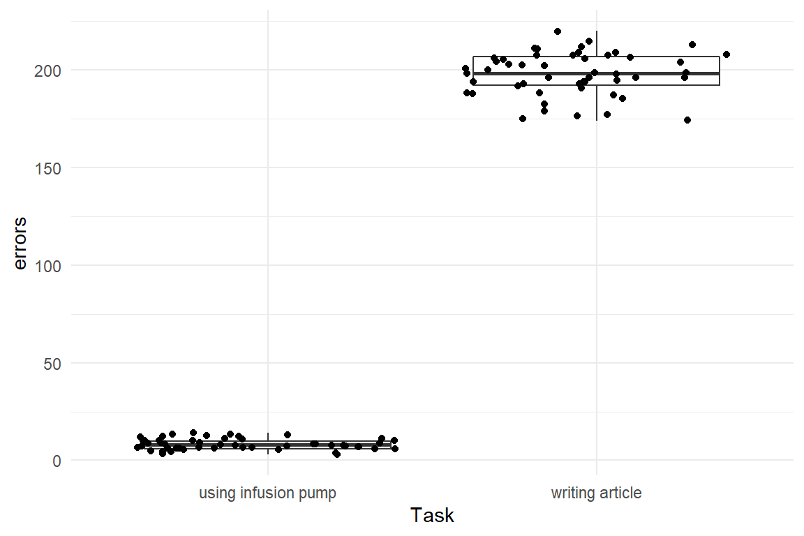
Figure 7.7: Mean-variance relationship of Poisson distributed data with two groups
Not by coincidence, practically all distributions with a lower boundary have variance increase with the mean. Distributions that have two boundaries, like binomial or beta distributions also have a mean-variance relationship, but a different one. For binomial distributed variables, mean and variance are determined as follows:
\[ \begin{aligned} Y &\sim \textrm{Binom}(p, k)\\ E(Y) &= p k\\ \textrm{Var}(Y) &= p (1-p) k\\ \textrm{Var}(Y) &= E(Y)(1-p) \end{aligned} \]
To see this, imagine a study that examines the relationship between user expertise (for the convenience on a scale of zero to one) and success rate on ten tasks. The result is a cigar-like shape, like in Figure 7.8. For binomial distributions, variance gets largest, when the chance of success is centered at \(p = .5\). This is very similar for other distributions with two boundaries, such as beta and logit-Gaussian distributions.
tibble(
  expertise = runif(1000, 0, 1),
  successes = rbinom(1000, 25, expertise)
) %>%
  ggplot(aes(x = expertise, y = successes)) +
  geom_point()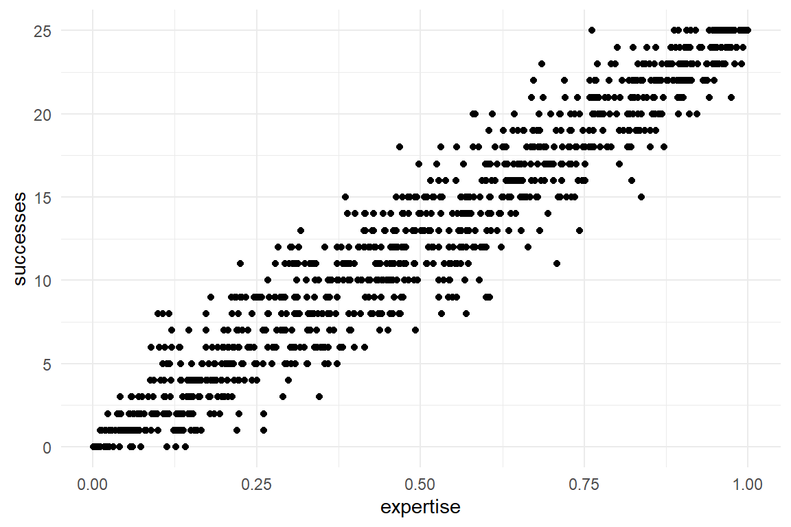
Figure 7.8: Cigar shaped mean-variance relationship of Binomial data
In conclusion, real distributions are typically asymmetric and have mean and variance linked. Both phenomena are tightly linked to the presence of boundaries. Broadly, the deviation from symmetry gets worse when observations are close to the boundaries (e.g. low error rates), whereas differences in variance is more pronounced when the means are far apart from each other.
Still, using distributions that are not Gaussian sometimes carries minor complications. Gaussian distributions have the convenient property that the amount of randomness is directly expressed as the parameter \(\sigma\). That allowed us to compare the fit of two models A and B by comparing \(\sigma_A\) and \(\sigma_B\). In random distributions with just one parameter, the variance of randomness is fixed by the location (e.g. Poisson \(\lambda\) or Binomial \(p\)). For distributions with more than one parameter, dispersion of randomness typically is a function of two (or more) parameters, as can be seen in the formulas above. For example, Gamma distributions have two parameters, but both play a role in location and dispersion.
Using distributions with entanglement of location and dispersion seems to be a step back, but frequently it is necessary to render a realistic association between location of fitted responses and amount of absolute randomness. Most distributions with a lower bound (e.g. Poisson, exponential and Gamma) increase variance with mean, whereas double bounded distributions (beta and binomial) typically have maximum variance when the distribution is centered and symmetric. For the researcher this all means that the choice of distribution family determines the shape of randomness and the relation between location and variance.
The following sections are organized by type of typical outcome variable (counts, durations and rating scales). Each section first introduces a one-parametric model (e.g. Poisson). A frequent problem with these models is that the location-variance relation is too strict. When errors are more widely dispersed than is allowed, this is called over-dispersion and one can either use a trick borrowed from multi-level models, observation-level random effects @(olre) or select a two-parametric distribution class (e.g., Negative-Binomial).
7.2 Count data
Gaussian distributions assume that the random variable under investigation is continuous. For measures, such as time, it is natural and it can be a reasonable approximation for all measures with fine-grained steps, such as average scores of self-report scales with a large number of items. Other frequently used measures are clearly, i.e. naturally, discrete, in particular everything that is counted. Examples are: number of errors, number of successfully completed tasks or the number of users. Naturally, count measures have a lower bound and sometimes this is zero (or can be made zero by simple transformations). A distinction has to be made, though, for the upper bound. In some cases, there is no well defined upper bound, or it is very large (e.g. number of visitors on a website) and Poisson regression applies. In other cases, the upper bound is determined by the research design. A typical case in design research is the number of tasks in a usability study. When there is an upper bound, Binomial distributions apply, which is called logistic regression.
7.2.1 Poisson regression
When the outcome variable is the result of a counting process with no obvious upper limit, Poisson regression applies. In brief, Poisson regression has the following attributes:
- The outcome variable is bounded at zero (and that must be a possible outcome, indeed).
- The linear predictor is on a logarithmic scale, with the exponential function being the inverse.
- Randomness follows a Poisson distribution.
- Variance of randomness increases linearly with the mean.
The link function is the logarithm, as it transforms from the non-negative range of numbers to real numbers (7.1.1). For a start, we have a look at a Poisson GMM. Recall the smart smurfer game from section 3.5.2.4. Imagine that in an advanced level of the game , items are well hidden from the player and therefore extremely difficult to catch. To compensate for the decreased visibility of items, every level carries an abundance of them. In fact, the goal of the designers is that visibility and abundance are so carefully balanced that, on average, a player finds three items. We simulate a data set for one player repeating the level 30 times (Figure 7.9) and run our first Poisson model, which is a plain GMM.
set.seed(6)
D_Pois <-
  tibble(
    Obs = 1:30,
    items_found = rpois(30, lambda = 3.4)
  )

D_Pois %>%
  ggplot(aes(x = items_found)) +
  geom_histogram()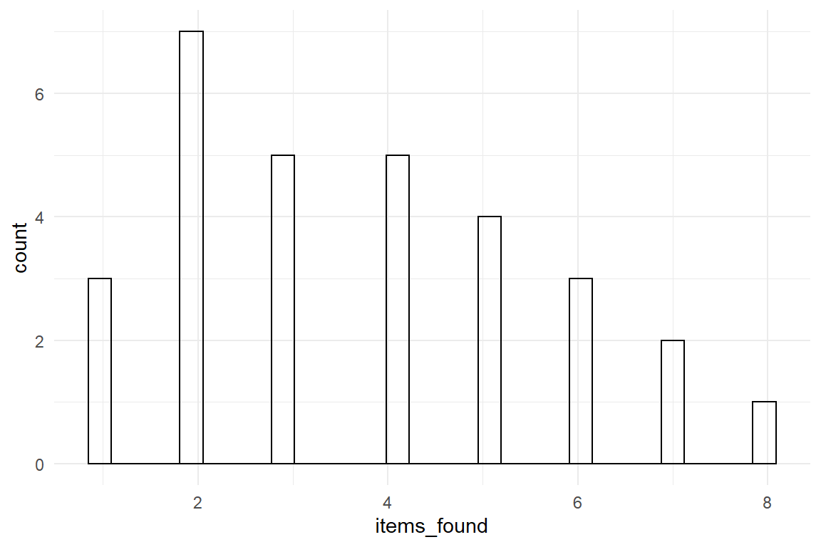
Figure 7.9: Data sampled from a Poisson distribution
M_Pois <-
  stan_glm(items_found ~ 1,
    family = poisson,
    data = D_Pois
)fixef(M_Pois)| model | type | fixef | center | lower | upper |
|---|---|---|---|---|---|
| object | fixef | Intercept | 1.31 | 1.12 | 1.49 |
Poisson distributions have only one parameter \(\lambda\) (lambda), which has a direct interpretation as the expected mean and variance of the distribution. On the contrary, the regression coefficient is on a logarithmic scale to ensure it has no boundaries. To reverse to the scale of measurement, we use the exponential function as the mean function 7.1.1:
fixef(M_Pois, mean.func = exp)| model | type | fixef | center | lower | upper |
|---|---|---|---|---|---|
| object | fixef | Intercept | 3.72 | 3.07 | 4.44 |
The exponentiated coefficient can now be interpreted as the expected number of items found per session. Together with the credibility limits it would allow the conclusion that the items are slightly easier to find than three per session. Before we move on to more complex Poisson models, let’s take a look of the formalism of the Poisson GMM:
\[ \begin{aligned} \theta_i &= \beta_0\\ \mu_i &= \exp(\theta_i)\\ y_i &\sim \textrm{Pois}(\mu_i) \end{aligned} \]
In linear models, the first equation used to directly relate fitted responses \(\mu_i\) to the linear term. As any linear term is allowed to have negative results, this could lead to problems in the last line, because Poisson \(\lambda\) is strictly non-negative. Linear predictor \(\theta_i\) is taking those punches from the linear term and hands it over to the fitted responses \(\mu_i\) via the exponential function. This function takes any number and returns a positive number, and that makes it safe for the last term that defines the pattern of randomness.
7.2.1.1 Speaking multipliers
To demonstrate the interpretation of coefficients other than the intercept (or absolute group means), we turn to the more complex case of the infusion pump study. In this study, the deviations from a normative path were counted as a measure for error-proneness. In the following regression analysis, we examine the reduction of deviations by training sessions as well as the differences between the two devices. As we are interested in the improvement from first to second session and second to third, successive difference contrasts apply (4.3.3).
attach(IPump)M_dev <-
stan_glmer(deviations ~ Design + session + session:Design +
(1 + Design + session | Part) +
(1 + Design | Task) +
(1 | Obs), ## observation-level ramdom effect
family = poisson,
data = D_pumps
)Note that in order to account for over-dispersion, observation-level random effect (1|Obs) has been used, see 7.2.3. For the current matter, we can leave that alone and inspect population-level coefficients (Table 7.5).
fixef(M_dev)| fixef | center | lower | upper |
|---|---|---|---|
| Intercept | 0.831 | 0.244 | 1.406 |
| DesignNovel | -1.555 | -2.364 | -0.785 |
| session | -0.234 | -0.335 | -0.133 |
| DesignNovel:session | -0.074 | -0.243 | 0.084 |
These coefficients are on a logarithmic scale and cannot be interpreted right away. By using the exponential mean function, we reverse the logarithm and obtain Table 7.6.
fixef(M_dev, mean.func = exp)| fixef | center | lower | upper |
|---|---|---|---|
| Intercept | 2.297 | 1.277 | 4.081 |
| DesignNovel | 0.211 | 0.094 | 0.456 |
| session | 0.791 | 0.715 | 0.876 |
| DesignNovel:session | 0.928 | 0.784 | 1.087 |
Like in the GMM, the intercept now has the interpretation as the number of deviations with the legacy design in the first session. However, all the other coefficients are no longer summands, but multiplicative. It would therefore be incorrect to speak of them in terms of differences.
\[ \begin{aligned} \mu_i &= \exp(\beta_0 + x_1\beta_1 + x_2\beta_2) \\ &= \exp(\beta_0) \exp(x_1\beta_1) \exp(x_2\beta_2) \end{aligned} \]
Actually, it is rather unnatural to speak of error reduction in terms of differences, as we did in previous chapters. If we would say “With the novel interface 1.8 fewer errors are being made,” that means nothing. 1.8 fewer than what? Instead, the following statements make perfect sense:
- In the first session, the novel design produces 2.297 times the deviations than with the legacy design.
- For the legacy design, every new training session reduces the number of deviations by factor 0.791
- The reduction rate per training session of the novel design is *92.843% as compared to the legacy design.
To summarize: reporting coefficients on the linearized scale is not useful. We are not tuned to think in logarithmic terms and any quantitative message would get lost. By applying the mean function, we get back to the original scale. As it turns out, what was a sum of linear terms, now becomes a multiplication. For this reason, Poisson regression has often been called a multiplicative model. Another name is log-linear model, which attests that on the log-scale the model is linear. As we will see next, that is perfectly true for the learning process: on the log scale, the training sessions in the IPump study are associated by a constant decrease in deviations from optimal path.
7.2.1.2 Linearizing learning curves
The Achilles heel of Gaussian linear models is the linearity assumption. All measures in this universe are finite, which means that all processes eventually hit a boundary. Linearity is an approximation that works well if you stay away from the boundaries. If you can’t, saturation effects happen and that means you have to add interaction effects or ordered factors to your model. Unless, you go multiplicative.
Classic Mechanics assumes that the a space rocket accelerates linearly with the energy production by its thrusters. Every Joule you burn increases your current speed \(\beta_0\) by \(\beta_1\) km/h. The problem with this assumption is that when you are already close to speed of light and the next thrust pushes you beyond the border. In the real world, \(E = Mc^2\) holds an every thrust increases the energy, and therefore also its drag, \(\beta_0\) is not constant. The advantage of multiplicative model is that it does not cross the boundary between positive and negative.
In the additive linear model, the learning curve is non-linear and we had to use an ordered factor model. Learning curves are characterized by running against an asymptote, which is the level of maximum level of achievable performance.
As we will see now, the clumsy OFM (4.3.5) can be replaced by a log-linear regression model, with just one slope coefficient. The idea of replacing the OFM with a *linear__ized__ regression model (LzRM), is attractive. For one, with such a model we can obtain valid forecasts* of the learning process. And second, the LzRM is more parsimonous 8.2.1. For any sequence length, an LzRM just needs two parameters: intercept and slope, whereas the OFM requires one coefficient per session.
As it happens, learning curves often follow the exponential law of practice. Basically, that means that the performance increase is defined as rate, rather than a difference. In a sentence that would be something like: Every training session reduces the number of errors by 20%. When initial errors are 100, then after \(n\) sessions it is:
ToT = \(100 \times .8^n\)
Exponential functions make pretty good learning curves and they happen to be the mean function of Poisson regression. This leads to the following simulation of a learning experiment. This simulation takes a constant step size of \(\log(.8) = -0.223\) on the log-linearized scale, resulting in a reduction of 20% per session.
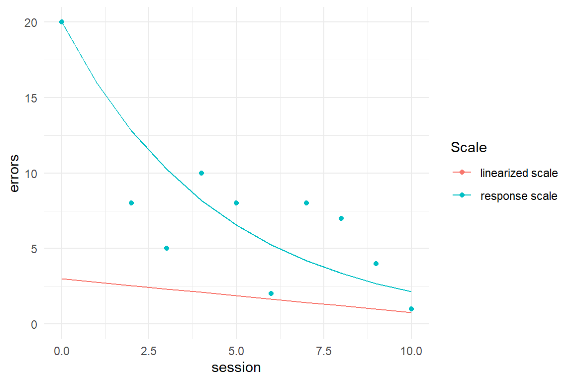
Figure 7.10: Exponential learning curve becoming linear under the log link function
While the linear predictor scale is a straight line, the response scale clearly is a curve-of-diminishing returns. That opens up the possibility that learning the novel pump design also has a constant difference on the linearized scale, which would mena a constant rate on the original scale. In the following, we estimate two Poisson models, one linearized OFM (OzFM) (with stairway dummies 4.3.5) and one LzRM. Then we will assess the model fit (using fitted responses). If the learning process is linear on the log scale, we can expect to see the following:
- The two step coefficients of the OzFM become similar (they were wide apart for ToT).
- The slope effect of the LzRM is the same as the step sizes.
- Both models fit similar initial performance (intercepts)
attach(IPump)D_agg <-
D_agg %>%
mutate(
Step_1 = as.integer(session >= 1),
Step_2 = as.integer(session >= 2)
)## Ordered regression model
M_pois_cozfm <-
D_agg %>%
brm(deviations ~ 0 + Design + Step_1:Design + Step_2:Design,
family = "poisson", data = .
)
## Linear regression model
M_pois_clzrm <-
D_agg %>%
brm(deviations ~ 0 + Design + session:Design, family = "poisson", data = .)For the question of a constant rate of learning, we compare the one linear coefficient of the regression model with the two steps of the ordered factor model (Figure 7.11):
T_fixef <-
  bind_rows(
    posterior(M_pois_cozfm),
    posterior(M_pois_clzrm)
  ) %>%
  fixef(mean.func = exp) %>%
  separate(fixef, into = c("Design", "Learning_unit"), sep = ":") %>%
  mutate(model = if_else(str_detect(model, "lz"),
    "Continuous Model", "Ordered Factor Model"
  )) %>%
  filter(!is.na(Learning_unit)) %>%
  arrange(Design, Learning_unit, model) %>%
  discard_redundant()

T_fixef %>%
  ggplot(aes(
    x = Learning_unit, y = center, col = Design,
    ymin = lower, ymax = upper
  )) +
  geom_crossbar(position = "dodge", width = .2) +
  facet_wrap(. ~ model, scales = "free_x") +
  labs(y = "rate of learning", scales = "free_x") +
  ylim(0, 1.2)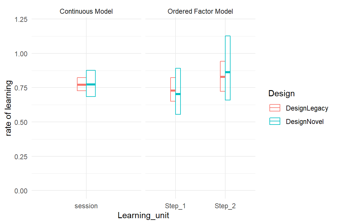
Figure 7.11: Learning rate estimates from a log-linearized continuous model and an OFM.
With the Poisson OFM the learning rates are very similar for both steps, which means the learning rate is almost constant and taking one learning step as a unit is justified. Furthermore, the learning rate appears to also be almost constant across designs. If that is true, one implication is that the novel design is superior in many aspects, accelerated learning may not be one of them. The other implication is that we no longer need two learning rate parameters (session). The final model in this section is the most simple one, it even no longer contains conditional effects. Table 7.7 can now be summarized in three simple sentences:
- On average there are 26 deviations with Legacy in the first session.
- Novel reduces deviations to 25% at every stage of learning.
- Per session, deviations are reduced by around 25%.
M_pois_lzrm <-
  D_agg %>%
  brm(deviations ~ 1 + Design + session,
    family = "poisson", data = .
)coef(M_pois_lzrm, mean.func = exp)| parameter | fixef | center | lower | upper |
|---|---|---|---|---|
| b_Intercept | Intercept | 26.250 | 24.508 | 27.989 |
| b_DesignNovel | DesignNovel | 0.247 | 0.221 | 0.276 |
| b_session | session | 0.773 | 0.731 | 0.815 |
For reporting results that is great news; you don’t have to explain ordinal factorial models or conditional effects and you can even tell the future to some extent. In 8.2.4, we will come back to this case and actually demonstrate that a unconditional model with two coefficients beats all the more complex models in predictive accuracy.
Normally, fitted responses are just retrospective. Here, we extrapolate the learning curve by fake data and obtain real forecasts. We can make more interesting comparison of the two devices. For example, notice that initial performance with Novel is around five deviations. With Legacy this level is reached only in the seventh session. We can say that the Novel design is always seven sessions of training ahead of Legacy.
The conclusion is that log-linearized scales can reduce or even entirely remove saturation effects, such that we can go with a simpler models, that are easier to explain and potentially more useful. Potentially, because we can not generally construct parametric learning curves with log-linear models. The crucial property here is that the lower bound is Zero. Some measures have a positive lower bound, which is constant and known, and can be translated to a lower bound of Zero. For example, path length, the minimum number of steps to find something on the internet is One, Path length can just shifted by One, e.g. mutate(addional_steps = steps + 1) to create a lower bound of Zero. This is different for Time-on-Task, which always has a strictly positive lower bound, which we don’t know and which probably varies between individuals. Learning curves that approach strictly positive asymptotes have the following mathematical form:
# devtools::install_github("schmettow/asymptote")
asymptote::ARY
## perf ~ ampl * exp(-rate * trial) + asym
## <environment: namespace:asymptote>The offset to Zero is in the summand asym, and because it is a summand this term cannot be linearized in a straight-forward manner. For general learning curves a truly non-linear model is required, not just a linearized. This can be constructed with the Brm engine, but is beyond the scope of this book.
7.2.2 Logistic (aka Binomial) regression
In the last section, we have seen how Poisson regression applies, when outcome variables are count numbers. More precisely, Poisson regression applies to count data, when there is no upper limit to counts (or if this limit is extremely large, as in the Smart Smurfer example). When the outcome variable is counts, but an upper limit exists and is known, logistic regression is an appropriate model. Such a situation often arises, when the counts are successes in a fixed number of trials. Logistic regression has the following properties:
- The outcome variable has a zero lower bound and a fixed upper bound, e.g. number of trials \(k\).
- The linear predictors are on a logit scale also called log-odds, which is reversed by a logistic function.
- The random component follows a binomial distribution.
- Due to the former, the variance of randomness is largest at \(\mu = 0.5\) or \(\eta = 1\) and declines towards both boundaries, taking a characteristic cigar shape.
Logistic regression applies for discrete outcomes, just like Poisson regression. The difference is that logistic regression has a finite number of possible outcomes, which is the number of trials plus one (no successes). In the following section, I will first introduce logistic regression for when there is only one trial per observation, with two possible outcomes. That is called dichotomous outcomes. Dichotomous outcomes are not limited to the Zero or One, Miss or Success, but apply to all outcomes that fall into two classes. In the subsequent section, we will look at logistic regression for when there is more than one trial. The most difficult part of logistic regression is to report the estimated coefficients in an intelligible manner, which will be covered in the final section.
7.2.2.1 Dichotomous outcomes
The most simple form of successes-in-trials measure is when there is only one trial. This is called a dichtotomous variable, and that is very common:
- a user is successful at a task, or fails
- a visitor returns to a website or does not
- a usability problem is discovered or remains unseen
- a driver brakes just in time or crashes
- a customer recommends a product to a friend or does not
- a user starts searching on a website by keyword or by traversing links
Often, dichotomous outcome variables have a quantitative notion in the sense of more or less desirable. When the outcome casts a positive light on the design, by convention it is coded as 1, otherwise 0. But, the dichotomy can also be two equal alternatives, such as whether a user starts a web inquiry by keyword search or by following a link. Let’s take this as an example.
Research on search strategies of web users revealed that they are quite ecclectic regarding their method to find a piece of information. In particular, most people use keyword search and link navigation at occasion. Web users are also known to be impatient companions, who build a first judgment very quickly and swiftly turn to a competitor’s site, when the first impression leaves something to be desired. Therefore, it can be valuable to know what method the majority of users prefer, initially.
For this purpose, we can classify users by what method they start with when given a search task during a usability study. As there exist only two options, keyword search or following links, we can capture the outcome in a dichotomous response variable. Below is the simulation of a small data set, where 40% of users initially prefer keyword search (Table 7.8)).
set.seed(42)
D_web <-
  tibble(init_keyword = rbinom(100, 1, .4)) %>%
  as_tbl_obs()

D_web| Obs | init_keyword |
|---|---|
| 18 | 0 |
| 21 | 1 |
| 24 | 1 |
| 40 | 1 |
| 55 | 0 |
| 57 | 1 |
| 69 | 1 |
| 82 | 0 |
For estimating the proportion of the two classes of users, we run a logistic regression grand mean model and inspect the coefficient table. Note that logistic regression is called so by its mean function (inverse link), not its shape of randomness. For counts with lower and upper border, the binomial family applies.
M_web <- stan_glm(init_keyword ~ 1,
  data = D_web,
  family = binomial
)clu(M_web)| parameter | fixef | center | lower | upper |
|---|---|---|---|---|
| Intercept | Intercept | -0.167 | -0.582 | 0.255 |
Clearly, the Intercept parameter is not a proportion, as that forbids negative values. Like with Poisson regression, the coefficient is on a linearized scale with infinite range. It is the logit functions that inflates the response range \(\mu_i \in [0;1]\) to the linear predictor linear predictor scale \(\eta_i \in [-\infty; \infty]\).
\[ \eta_i = \textrm{logit}(\mu_i) = \log \frac{\mu_i} {1-\mu_i} \]
Note that the fraction \(\frac{\mu_i} {1-\mu_i}\) is the proportion of keyword search divided by the proportion of following links and is called an odds. The logit function is therefore often called log-odds. In section 7.2.2.3, we will see how we can report logistic regression results as odds. In the case of our simple GMM, we can directly report the results as proportions, which requires to apply the mean function, which is the inverse of the logit, also known as the logistic function:
\[ \mu_i = \textrm{logit}^{-1}(\eta_i) = \frac{\exp \eta_1} {\exp \eta_i + 1} \]
In GMM, \(\eta_i = \beta_0\) and we can directly obtain the estimated proportion by applying the logistic function to the Intercept. The clu command lets you pass on a mean function, resulting in Table 7.10.
posterior(M_web) %>% clu(mean.func = inv_logit)| parameter | fixef | center | lower | upper |
|---|---|---|---|---|
| Intercept | Intercept | 0.458 | 0.359 | 0.563 |
From the GMM we retrieve one estimate that reflects the proportion to start by keyword search. That works for absolute group mean, but most of the time, logistic regression coefficients are exponentiated and read as odds 7.2.2.3.
As a side note, proportions could also be called probabilities, like “with 40% probability a user starts by keyword search.” However, I urge anyone to avoid speaking of logistic regression coefficients as probabilities. While mathematically this is correct, for the audience it can easily cause confusion with certainty or, beware of this, the p-value.
The apt reader may have noticed that the returners data set has been simulated with an exact return rate of 40%. Despite the sample size of 100, the center estimate seems rather off and hampered by considerable uncertainty. In computer science jargon, every dichotomous observation accounts to a bit, which is the smallest amount of information possible. Because the information of a single dichotomous observation is so sparse, large samples are important when dealing with dichotomous outcomes. Large samples can mean testing many users, or giving every user more than one trial.
7.2.2.2 Successes in a number of trials
If we repeatedly observe a dichotomous response, we can summarize the results as successes-in trials, like:
responses <- c(0, 1, 1, 1, 0, 1)
cat(sum(responses), "successes in", length(responses), "trials")
## 4 successes in 6 trialsImagine we had conducted an extended version of the previous experiment, where users get set of ten tasks and we observe their initial behavior every time they open a new website. As such tasks sometimes take very long, it may also happen that a participant cannot finish all ten tasks within time. That means, we potentially have a different number of attempts per participant, which we simulate as Binomial random numbers (Table 7.11).
set.seed(42)
D_web_ex <-
  tibble(
    trials = round(runif(100, 7, 10), 0),
    init_keyword = rbinom(100, trials, .4),
    init_link = trials - init_keyword
  ) %>%
  mascutils::as_tbl_obs()

D_web_ex| Obs | trials | init_keyword | init_link |
|---|---|---|---|
| 14 | 8 | 3 | 5 |
| 24 | 10 | 4 | 6 |
| 25 | 7 | 4 | 3 |
| 34 | 9 | 6 | 3 |
| 61 | 9 | 6 | 3 |
| 62 | 10 | 4 | 6 |
| 92 | 7 | 4 | 3 |
| 98 | 9 | 2 | 7 |
In order to estimate a model on the proportion of successes in a number of trials, somehow this needs to be specified. That is done indirectly via the number of “failures,” in this case this is the number of times a link was followed, rather than a search query. The response side of the model formula takes this in as an array with two columns, which is generally constructed as cbind(successes, failures). We estimate a Binomial GMM and extract the coefficient as a proportion (Table 7.12):
M_web_ex <- stan_glm(cbind(init_keyword, init_link) ~ 1, # <--
  family = binomial,
  data = D_web_ex
)fixef(M_web_ex,
mean.func = inv_logit
)| model | type | fixef | center | lower | upper |
|---|---|---|---|---|---|
| object | fixef | Intercept | 0.406 | 0.374 | 0.442 |
With a ten-fold of data, as compared to the dichotomous model, the estimate is much closer to the real value and the credibility intervals tightened up, too. By using the inverse logit, we can readily report the results as proportions. Again, make no mistake, this really only works for GMMs and AMMs. when effects come into play and additional coefficients are being estimated, reporting proportions does no longer work. Instead, we have to learn to talk odds.
Recall, how we characterized tasks as populations and introduced multi-level models with task-level coefficients (6.5). It could appear as if a multiple-trials Binomial model is an alternative to multi-level modeling. It is not! First of all, there are no task-level estimates. In contrast, the above model assumes that chance of success is constant across tasks. If these are not simple experimental tasks, all quite the same, this assumption most is violated. More specifically, recall that the variance of Binomial distributions is fixed by the mean. If tasks vary, this will create over-dispersion ((7.2.3)).
7.2.2.3 Talking odds
When presenting results of a statistical analysis, the linear predictor is likely to cause trouble, at least when the audience is interested in real quantities. Especially Coefficients on a logit-linearized scale have only very general intuition:
- zero marks a 50% chance
- positive values increase the chance, negative decrease
- bigger effects have larger absolute values
That is sufficient for purely ranking predictors by relative impact (if on a comparable scale of measurement), or plain hypothesis testing, but it does not connect well with quantities a decision maker is concerned with. Let’s see this at the example of the infusion pump study, where some relevant questions for the evaluation of failures are
- What is the expected frequency of failure on first use?
- The novel design reduces failures, but is it sufficient?
- Is frequency of failures sufficiently reduced after two training sessions?
In the comparison of two medical infusion pumps (@ref(slope_RE)) 25 nurses completed a set of eight tasks repeatedly over three sessions. In @ref(slope_RE) a multi-level model was estimated on the workload outcome. It is tempting to apply the same structural model to success in task completion, using binomial random patterns and logit links.
completion ~ Design*Session + (Design*Session|Part) + (Design*Session|Task)Such a model is practically impossible to estimate, because dichotomous variables are so scarce in information. Two populations encounter each other in the model: participants and tasks, with 6 observations per combination (6 bit). We should not expect to get reasonably certain estimates on that level and, in fact, the chains will not even mix well. The situation is a little better on the population level: every one of the six coefficients is estimated on 400 bit of raw information. We compromise here by estimating the full model on population level and do only intercept random effects to account for gross differences between participants and tasks (Table 7.13).
attach(IPump)M_cmpl <-
D_pumps %>%
stan_glmer(completion ~ Design * Session +
(1 | Part) + (1 | Task),
family = binomial,
data = .
)fixef(M_cmpl)| fixef | center | lower | upper |
|---|---|---|---|
| Intercept | 1.317 | 0.131 | 2.522 |
| DesignNovel | 0.403 | 0.080 | 0.719 |
| Session2-1 | 0.692 | 0.138 | 1.237 |
| Session3-2 | -0.079 | -0.635 | 0.457 |
| DesignNovel:Session2-1 | -0.301 | -1.093 | 0.494 |
| DesignNovel:Session3-2 | 0.286 | -0.546 | 1.079 |
The result is one absolute group mean, the Intercept, and five effects, which are mean differences on the logit-linearized scale \(\eta_i\). If we want to report absolute group means, we can use the inverse logit function to obtain proportions, but for that we have to first do the linear combination followed by the transformation, for example:
- the completion rate in the first legacy session is 0.789
- in novel/session 1:
logist(Intercept + DesignNovel)= 0.848 - in novel/session 2:
logist(Intercept + DesignNovel + Session2-1 + DesignNovel:Session2-1)= 0.892 - in legacy/session 3:
logist(Intercept + DesignNovel + Session2-1)= 0.873
Above we have used the inverse-logit (aka logistic) mean function to elevate the absolute group means to proportions. This is an intuitive scale, but unfortunately, the mean function does not apply to individual effects. It is for example, incorrect to apply it like: “the novel pumps proportion of failures in the first session increases by logist(DesignNovel) = 0.6.”
Log-odds are compound function. The inner part of the function, the odds, are the chance of success divided by the chance of failure. Especially in the anglo-american culture, odds are a rather common way to express ones chances in a game, say:
- odds are 1 against 1 that the coin flip produces Head. If you place €1 on Head, I put €1 on tail.
- odds are 1 against 12 that Santa wins the dog race. If you place 1€ on Santa, I place €12 against.
- 46% on Red. 54% on Blue
Reversing only the logarithm produces odds, as in Table 7.14
fixef(M_cmpl, mean.func = exp)| fixef | center | lower | upper |
|---|---|---|---|
| Intercept | 3.733 | 1.140 | 12.45 |
| DesignNovel | 1.497 | 1.083 | 2.05 |
| Session2-1 | 1.999 | 1.148 | 3.44 |
| Session3-2 | 0.924 | 0.530 | 1.58 |
| DesignNovel:Session2-1 | 0.740 | 0.335 | 1.64 |
| DesignNovel:Session3-2 | 1.331 | 0.579 | 2.94 |
But is it legitimate to apply the transformation on individual coefficients in order to speak of changes of odds? The following arithmetic law tells that what is a sum on the log-odds scale, is multiplication on the scale of odds:
\[ \exp(x + y) = \exp(x)\exp(y) \]
Consequently, we may speak of changes of odds using multiplicative language:
- If you place €100 on failure in the next task with the legacy design in session 1, I place €373.303 on success.
- The odds of success with the novel design increase by factor 1.497. Now, I would place \(373.303 \times 1.497\) = €558.835 on success.
- On success with the novel design in session 2, I would place \(373.303 \times 1.497 \times 1.999 \times 0.74\) = €826.809 on success.
Once, we have transformed the coefficients to the odds scale, we can read coefficients as multipliers and speak of them in hard currency.
To summarize: Logistic regression applies when the basic observations falls into two classes. For any research design involving such outcomes, repetition is highly recommended, and outcomes can be summarized into successes-in-trials. Reporting coefficients on the logit scale is only useful when nobody is interested in intelligible effects sizes. How to report the results depends on the research question. If one is interested in proportions per group, the inverse logit applies to the absolute group means and this can be easily understood. If one wants to talk about effects or differences, such as the amount of improvement with a novel design, only the logarithm is reversed, and effects are reported as odds. Depending on the audience, this may be more or less intuitive, but it can always be embedded in a wager for illustration.
Logistic regression is known in many areas of application, as well as for some interesting extensions.
- In epidemiology research, logistic regression is the indispensable tool for several central outcomes, such as hospitalization, mortality, infection and recovery.
- In psychometrics, the famous Rasch model applies for measuring a persons ability by the number of correct answers in a test. A Rasch model is just a cross-classified multilevel logistic regression 6.8.4.
- If the outcome is a classification with more than two classes, multi-nomial regression is an extension of logistic regression.
- In section 4.3.5, we will encounter ordinal logistic regression, which applies for classifications with an order, such as responses on Likert scales.
One frequent problem when using logistic regression on successes-in-trials outcomes is that the assumption of a Binomial shape of randomness is violated by over-dispersion. Like Poisson distributions, Binomial distributions have a variance tightly linked to the mean, but frequently there is more variance than allowed, for example when tasks or test items vary in difficulty. In the following section two solutions to the problem are introduces: beta-binomial regression and observation-level random effects.
7.2.3 Modelling overdispersion
Poisson and binomial distributions are one-parameter distributions. As there is only one parameter, it is impossible to choose location and dispersion independently. In effect, both properties are tightly entangled. For Poisson distributions they are even the same.
\[ \begin{aligned} Y &\sim \textrm{Poisson} (\lambda) \\ \textrm {Var}(Y) &= \textrm {Mean}(Y) = \lambda \end{aligned} \]
For binomial distributions, mean and variance both depend on probability \(p\) and are entangled in cigar shaped form, as the dispersion shrinks when approaching the lower or upper boundaries. Binomial variance is also affected by the number of trials \(k\), but that hardly matters as the value of \(k\) is usually not up for estimation, but known.
\[ \begin{aligned} Y &\sim \textrm{Binom} (p, k) \\ \textrm {Mean}(Y) &= kp \\ \textrm {Var}(Y) &= kp(1 - p) \\&= \textrm {Mean}(Y) (1-p)\\ \end{aligned} \]
In real data, we often see similar relationships between variance and mean, except that variance is inflated by some additional positive factor, which is called overdispersion. Poisson or Binomial distribution cannot render inflated data, and using them on over-dispersed data is a serious mistake. Fortunately, there exist two solutions to the problem, which I will introduce in the following three sections. In the first two sections, we will replace the one-parameter distribution with a two-parameter distribution, where the second parameter represents the variance inflation. The second method is to use observation-level random effects, which draws from the multi-level modeling toolbox.
Let me give you an example to illustrate the two methods. It is common saying that some people attract mosquito bites more than others. But is that really true? A simple lab experiment could be done to test the “Sweet Blood” theory. A sample of participants are exposed to a pack of mosquitoes under carefully controlled conditions (time of day, environmental condition, hungriness of mosquitoes). We don’t know the mechanisms that makes the blood sweeter, and hence cannot measure it. In the simulation below, it is just assumed that there is a such a property, but in a real study we would not know.
The following simulation function works by using a two-parameter distribution, that have the same properties as Poisson (or binomial) distributions. Negative-binomial distributions are discrete distributions with a lower bound of zero, just like Poisson distributions. They also have the same location parameter \(\mu\), but a new parameter size, which re-scales the scale of measurement. When the scale of measurement is down-scaled, the distribution becomes relatively wider. When size approaches infinity, we are left with a plain Poisson variance. The following data simulation samples Sweet-blood data from a negative-binomial distribution with a size of 3 (Table 7.15).
set.seed(42)
N <- 400
avg_sweet <- 6
size <- 3

Sweet_blood_nbin <- tibble(
  Method = "NegBinomial",
  bites = rnbinom(
    n = N,
    mu = avg_sweet,
    size = size
  )
)

Sweet_blood_nbin %>%
summarize(mean(bites), var(bites)) | mean(bites) | var(bites) |
|---|---|
| 6 | 19.2 |
The next simulation first creates an observation-level score for blood sweetness, which in real data would not be known to the researcher; it is therefore similar to a random effect. A property called Sweetness is first sampled from a Gaussian distribution. The result is exponentiated to achieve positive numbers and plugged into the Poisson random number generator. Table 7.16 shows how variance exceeds the mean of the so the produced responses.
set.seed(42)
sd <- .5


Sweet_blood_olre <-
  tibble(
    Method = "OLRE",
    sweetness = rnorm(N, mean = log(avg_sweet), sd = sd),
    bites = rpois(N, lambda = exp(sweetness))
  )

Sweet_blood_olre %>%
summarize(mean(bites), var(bites)) | mean(bites) | var(bites) |
|---|---|
| 6.67 | 20.3 |
tibble(
  Method = "Poisson",
  bites = rpois(N, avg_sweet)
) %>%
  bind_rows(
    Sweet_blood_nbin,
    Sweet_blood_olre
  ) %>%
  ggplot(aes(x = bites)) +
  geom_histogram() +
  facet_grid(Method ~ .)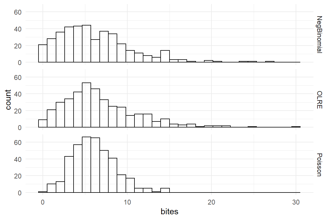
Figure 7.12: Overdispersed samples (Negbinomial, OLRE) compared to Poisson samples of same average.
When building a model for over-dispersed count data, the process of simulating it is simply reversed, for both methods. Either we choose a more flexible distribution, or we estimate the residuals on the linearized scale. The first method has the advantage of being leaner. Only one parameter is added, whereas OLRE results in one linearized residual for every observation. The advantage of OLRE is more of a conceptual kind. Not only is it appealing for researchers who are familiar with multi-level models, it also produces estimates similar to the well-known residuals. Furthermore, it also works with regression engines that do not cover the two-parameter distribution. In fact, the beta-binomial family is the matching two-parameter distribution for Binomial variables, but is not supported out-of-the-box by any regression engine I am aware of. In 7.2.3.2, we will see how user-defined distributions can be added to the Brm engine.
–>
7.2.3.1 Negative-binomial regression for overdispersed counts
When Poisson regression is used for overdispersed count data, the model will produce accurate center estimates, but the credibility limits will be too narrow. The model suggests better certainty than there is. To explain that in simple terms: The model “sees” the location of a measure, which makes it seek errors in a region with precisely that variance. There will be many measures outside the likely region, but the model will hold on tight, regard these as (gradual) outliers and give them less weight. A solution to the problem is using a matching response distribution with two parameters. A second parameter usually gives variance of the distribution more flexibility, although only Gaussian models can set it completely independent of location.
In 7.2.1.2 we have seen how log-linearization can accommodate learning curves, using a Poisson model. It is very likely that this data is over-dispersed and that the Poisson model was not correct. To demonstrate overdispersion, we estimate the linearized learning curve one more time, with a negative-binomial pattern of randomness. Figure 7.13 shows the coefficient estimates next to coefficients from the Poisson model
attach(IPump)M_negbin_lzrm <-
brm(deviations ~ 1 + Design + session,
data = D_agg,
family = "negbinomial"
)bind_rows(
posterior(M_pois_lzrm),
posterior(M_negbin_lzrm)
) %>%
filter(type == "fixef") %>%
clu() %>%
ggplot(aes(y = center, ymin = lower, ymax = upper, x = model)) +
facet_wrap(~fixef, scales = "free_y") +
geom_crossbar(position = "dodge")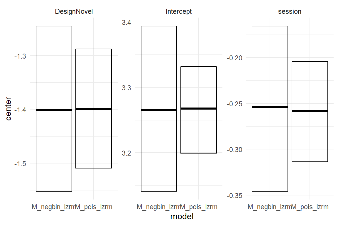
Figure 7.13: Comparing credibility intervals of a Poisson and Neg-Binomial models
We observe that the center estimates are precisely the same. Over-dispersion usually does not bias the location of an estimate. But, credibility limits are much wider with an underlying negative-binomial distribution. A full parameter table would also show the Neg-Binomial model additional parameter phi, controlling over-dispersion relative to a Poisson distribution as:
\[ \textrm{Variance} := \mu + \mu^2/\phi \]
Due to the reciprocal term, the smaller \(\phi\) gets, the more overdispersion had to be accounted for. From this formula alone it may seem that neg-binomial distributions could also account for under-dispersion, when we allow negative values. But, in most implementations \(\phi\) must be non-negative. That is rarely a problem, as under-dispersion only occurs under very special circumstances. Over-dispersion in count variables in contrast, is very common, if not ubiquitous. Negative-binomial regression solves the problem with just one additional parameter, which typically need not be interpreted. Reporting on coefficients uses the same principle as in plain Poisson regression: inversion by exponentiation and speaking multiplicative.
7.2.3.2 Beta-binomial regression for successes in trials
Beta-binomial regression follows a similar pattern as negative-binomial. A two parameter distribution allows to scale up the variance relative to a binomial model 7.2.2. A beta-binomial distribution is a mixed distribution, created by replacing binomial parameter \(p\) by a \(beta distribution\), with parameters \(a\) and \(b\):
rbetabinom <- function(n, size, a, b) {
  rbinom(n, size, rbeta(n, a, b))
}

rbetabinom(1000, 10, 1, 2) %>% qplot()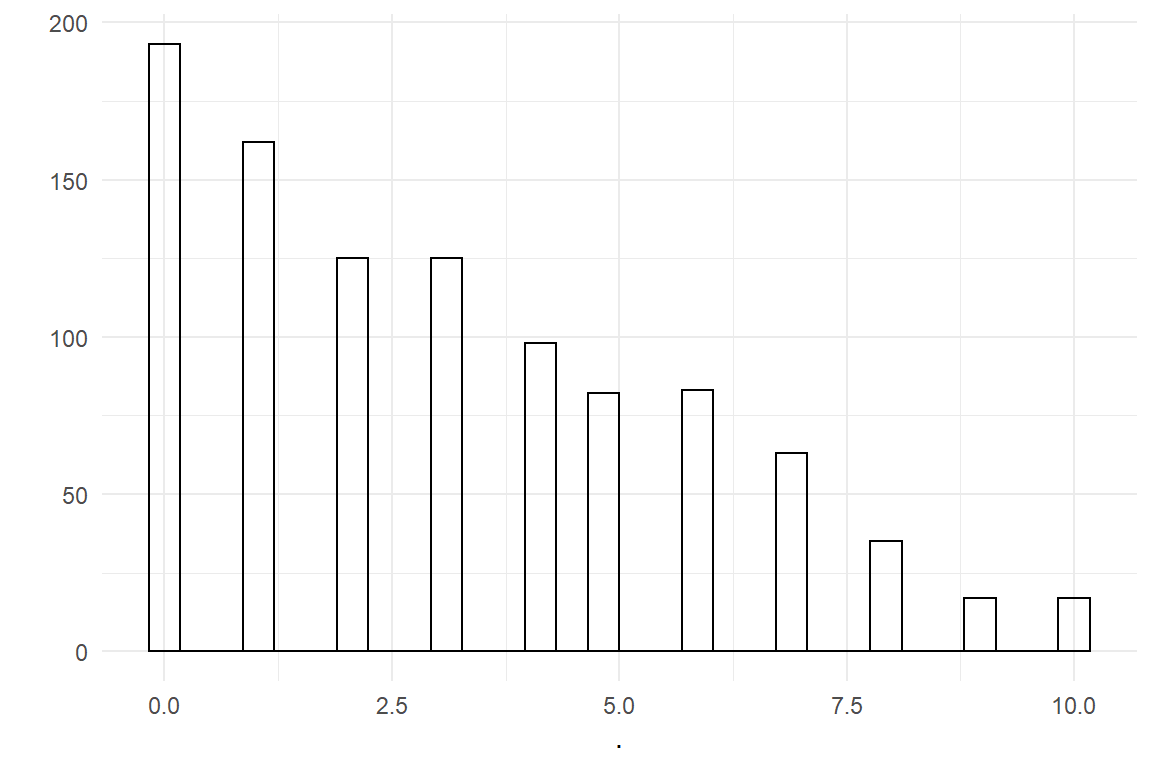
Figure 7.14: Sampling from a Beta-Bionomial distribution
The Brms regression engine currently does not implement the beta-binomial family. That is a good opportunity to applaud the author of the Brms package for his ingenious architecture, which allows custom families to be defined by the user. The only requirement is that the distribution type is implemented in Stan (Carpenter et al. 2017), which is the underlying general-purpose engine behind Brms. The following code is taken directly from the Brms documentation and adds the beta-binomial family.
# define a custom beta-binomial family
beta_binomial2 <- custom_family(
  "beta_binomial2",
  dpars = c("mu", "phi"),
  links = c("logit", "log"), lb = c(NA, 0),
  type = "int", vars = "trials[n]"
)

# define custom stan functions
bb_stan_funs <- "
  real beta_binomial2_lpmf(int y, real mu, real phi, int N) {
    return beta_binomial_lpmf(y | N, mu * phi, (1 - mu) * phi);
  }
  int beta_binomial2_rng(real mu, real phi, int N) {
    return beta_binomial_rng(N, mu * phi, (1 - mu) * phi);
  }
"
Note that Beta-binomial distribution are usually parametrized with two shape paramneter \(a\) and \(b\), which have a rather convoluted relationship with mean and variance. For a GLM a parametrization is required that has a mean parameter (for \(\mu_i\)). Note, how the author of this code created a beta_binomial2 distribution family, which takes \(\mu\) and a scale parameter \(\phi\).
Defining the two functions is sufficient to estimate beta-binomial models with Brms. In the following I simulate two outcomes from nine trials, y is sampled from a beta-binomial distribution, whereas ybin is from a Binomial distribution. Both have the same mean of \(.1\) (10% correct). Subsequently, a beta-binomial and a binomial grand mean models are estimated. Note that the sampling function is taken from package VGAM, as this has the same parametrization.
set.seed(42)
D_betabin <- tibble(
  y = VGAM::rbetabinom(1000, 9, prob = .1, rho = .3),
  n = 9
) %>%
  as_tbl_obs()

M_betabin <-
  D_betabin %>%
  brm(y | trials(n) ~ 1,
    family = beta_binomial2,
    stan_funs = bb_stan_funs, data = .
  )

M_bin <- brm(y | trials(n) ~ 1, family = "binomial", data = D_betabin)
The following CLU table collects the estimates from both models, the true beta-binomial and the binomial, which does not account for over-dispersion in the data.
bind_rows(
  posterior(M_bin),
  posterior(M_betabin)
) %>%
clu(mean.func = inv_logit)| model | parameter | fixef | center | lower | upper |
|---|---|---|---|---|---|
| M_betabin | b_Intercept | Intercept | 0.104 | 0.093 | 0.116 |
| M_betabin | phi | 0.927 | 0.893 | 0.955 | |
| M_bin | b_Intercept | Intercept | 0.103 | 0.097 | 0.110 |
When comparing the two intercept estimates, we notice that the center estimate is not affected by over-dispersion. But, just like with Poisson models, the binomial model is too optimistic about the level of certainty.
To summarize: one-parameter distributions usually cannot be used to model count data due to extra variance. One solution to the problem is to switch to a family with a second parameter. These exist for the most common situations. When we turn to modeling durations, we will use the Gamma family to extend the Exponential distribution 7.3.1. Gamma distributions have another problem: while extra variance can be accounted by a scale parameter, we will see that another property of distribution families can be to rigid, the skew. The solution will be to switch to a three-parameter distribution family to gain more flexibility.
Another technique to model over-dispersion does not require to find (or define) a two-parametric distribution. Instead, observation-level random effects borrow concepts from multi-level modeling and allow to keep the one-parameter distributions.
7.2.3.3 Using observation-level random effects
As we have seen in chapter 6, random effects are often interpreted towards variance in a population, with a Gaussian distribution. On several occasions we used multi-level models to separate sources of variance, such as between teams and participants in CUE8 (@ref()). Observation-level random effect (OLRE) use the same approach by just calling the set of observation a population.
Using random effects with GLMs is straight-forward, because random effects (or their dummy variable representation, to be precise), are part of the linear term, and undergo the log or logit linearization just like any other coefficient in the model.
For demonstration of the concept, we simulate from an overdispersed Poisson grand mean model with participant-level variation and observation-level variation.
sim_ovdsp <- function(beta_0 = 2, # mu = 8
                      sd_Obs = .3,
                      sd_Part = .5,
                      N_Part = 30,
                      N_Rep = 20,
                      N_Obs = N_Part * N_Rep,
                      seed = 1) {
  set.seed(seed)
  Part <- tibble(
    Part = 1:N_Part,
    beta_0p = rnorm(N_Part, 0, sd_Part)
  ) ## participant-level RE
  D <- tibble(
    Obs = 1:N_Obs,
    Part = rep(1:N_Part, N_Rep),
    beta_0i = rnorm(N_Obs, 0, sd_Obs), ## observeration-level RE
    beta_0 = beta_0
  ) %>%
    left_join(Part) %>%
    mutate(
      theta_i = beta_0 + beta_0p + beta_0i,
      mu_i = exp(theta_i), ## inverse link function
      y_i = rpois(N_Obs, mu_i)
    )
  D %>% as_tbl_obs()
}

D_ovdsp <- sim_ovdsp()
The above code is instructive to how OLREs work:
- A participant-level random effect is created as
beta_0p. This random effect can be recovered, because we have repeated measures. This variation will not contaminate Poisson variance. - An observation-level random effect is created in much the same way.
- Both random effects are on the linearized scale. The linear predictor
theta_iis just the sum of random effects (and Intercept). It could take negative values, but … - … applying the inverse link function (
exp(theta_i)) ensures that all responses are positive.
The extra variation comes from two sources: participant-level and observation-level. While participant levels, observations do not. How does come that we can estimate random effects on single measures? Recall that one-parameter distributions, such as Poissons, have their variance fully tied to the mean. At any position does the distribution “know” how much variance it is suppose to have and therefore the OLREs can be recovered. The following model contains an participant-level random effects and an OLRE. Table 7.18 recovers the two standard deviations.
M_ovdsp <-
  D_ovdsp %>%
  stan_glmer(y_i ~ 1 + (1 | Part) + (1 | Obs),
    data = .,
    family = poisson
)grpef(M_ovdsp)| re_factor | center | lower | upper |
|---|---|---|---|
| Obs | 0.330 | 0.289 | 0.373 |
| Part | 0.503 | 0.387 | 0.683 |
Let’s first take a look at the two random effect standard errors above. It seems that we got a fair recovery on the center estimates (for standard deviation). For the OLRE certainty is also good, even better than for the participant-level, which is simply due to the fact that there are more levels. Random effect variation is accurately recovered from the simulated data, but can we also recover the full vector of factor levels? In the following I am extracting observation-level random effects and plot them against the simulated (linearized) coefficients.
OLRE <-
  posterior(M_ovdsp) %>%
  filter(type == "ranef", re_factor == "Obs") %>%
  clu()

D_ovdsp %>%
  bind_cols(OLRE) %>%
  select(true_score = beta_0i, olre = center) %>%
  ggplot(aes(x = true_score, y = olre)) +
  geom_point() +
  geom_smooth(method = "lm", se = F)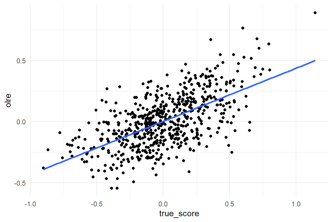
Figure 7.15: Recovery of observation-level random effects
Figure 7.15 shows that the observation-level deviations can be recovered not perfectly, but to some extent. An OLRE can be seen as generalized residual, or linearized residuals.
Linearized residuals can be used for different purposes, such as outlier detection or to compare sources of variation. Frequently, I reminded the reader to interpret parameters quantitatively by translating their magnitude to statements of practical relevance. For random effects variance this is not always straight forward, especially when we are on a linearized scale. One way is to make comparative statements on the sources of variance, like “the variance due to individual differences exceeds the measurement error.” OLREs are on the same scale as all other random effects in the model, which makes it a suitable reference source of variation.
## [1] "sim_ovdsp" "D_ovdsp"7.3 Duration measures
Time is a highly accessible measure, as clocks are all around us: on your wrist, in transport stations, in your computers and a very big (and accurate) one is hosted at the Physikalisch-Technischen Bundesanstalt in Braunschweig (Physical-technological federal institute in Braunschweig, Germany). Duration measures often carry useful information; especially, Reaction time (RT) measures are prime in experimental cognitive studies and have revealed fascinating phenomena of the human mind, such as the Stroop effect, memory priming, motor learning and the structure of attention.
In design research, reaction times are also sometimes used in experiments, but more common is time-on-task (ToT) as a measure of task efficiency. Formally, both outcome types measure a period of time. I am deliberately making a distinction between the two, because the data generating process of reacting to a simple task (like naming a color) may be different to a complex task, like finding information on a website. Also, RT and ToT usually are on different scales, with RT being typically in the fraction-of-seconds range and ToT in the minutes range.
Temporal variables are practically continuous (as long as one measures with sufficient precision), but always have lower bounds. First, I will introduce two families of zero-bounded model classes that use exponentially or Gamma distributed error terms. Modern Bayesian estimation engines offer an increasing variety of more exotic response distributions. Among those are Exgaussian response distributions, which works well when the lower bound is positive. Normally, this is more realistic for durations.
7.3.1 Exponential and Gamma regression
Exponential distributions arise from basic random processes under some very idealized conditions. First, the lower boundary must be zero and second, the rate at which events happen is assumed to be constant rate, just like Poisson distributions assumes a constant \(\lambda\).
Reconsider the subway smurfer example 3.5.2, where players collect items in a jump-and-run game. We have already seen how collection counts can be modeled using Poisson or binomial regression. Another way to look at it is the time between two events of item collection. For demonstration only, we assume such idealized conditions in the subway smurfer example and generate a data set. Exponential distributions are determined by one parameter, the rate parameter \(\lambda\), which is strictly positive. The mean and variance of exponential distributions are as follows, and they are strictly tied to each other:
\[ \begin{aligned} Y &\sim \textrm{Exp} (\lambda) \\ \textrm {Mean}(Y) &= 1/\lambda \\ \textrm {Var}(Y) &= 1/\lambda^2\\ &= 1/\lambda \times \textrm{Mean}(Y)\\ \end{aligned} \]
In the following, data is simulated from an exponential distribution (Figure 7.16). Subsequently, the only parameter is recovered using an exponential GMM. Like for Poisson models, a log link function is reversed by exponentiation (Table 7.19).
set.seed(20)
D_exp <-
  tibble(
    Obs = 1:100,
    time = rexp(100, rate = 1 / 3)
  )

D_exp %>%
  ggplot(aes(x = time)) +
  geom_histogram(bins = 20)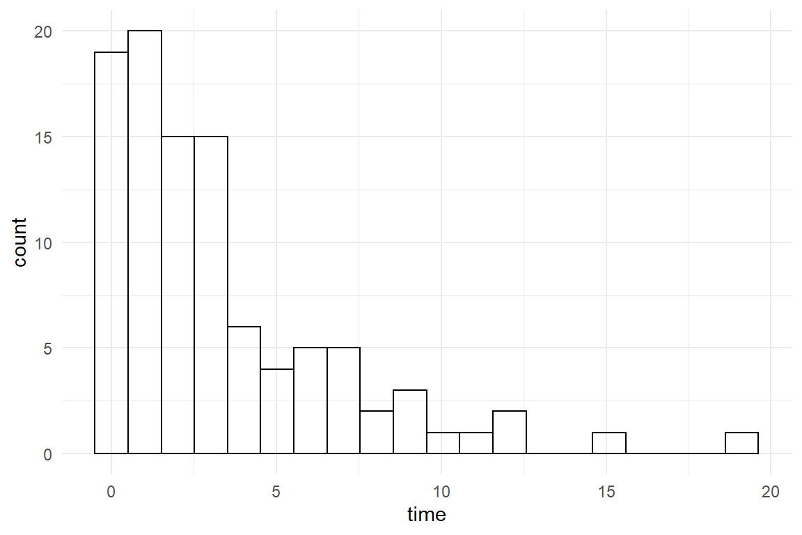
Figure 7.16: Data sampled from an Exponential distribution.
M_exp <- brm(time ~ 1,
  family = "exponential",
  data = D_exp
)clu(M_exp, mean.func = exp)| parameter | fixef | center | lower | upper |
|---|---|---|---|---|
| b_Intercept | Intercept | 1.19 | 1 | 1.38 |
| lp__ | -221.24 | -223 | -221.02 |
Exponential distribution are rarely used in practice for two shortcomings: first, the strict mean-variance relation makes it prone to over-dispersion. This can be resolved by using observation-level random effects 7.2.3.3 or using Gamma distributions, which accounts for extra variance by a second parameter. The second problem is the lower boundary of Zero, which will later be resolved by using Exgaussian error distributions (7.3.2).
Exponential regression has a single parameter and therefore has the same problem as seen with Poisson and binomial regression before. Only if all events have the same rate to occur, will an exponential distribution arise, which means for behavioral research: never. A general solution to the problem is introducing an observation-level random effect 7.2.3.3. Here, I will we will tackle the problem by using continuous, zero-bounded mixture distributions with two parameters, the Gamma family of distributions.
The canonical form of Gamma distribution uses two parameters rate and shape, which do not directly translate into location and dispersion. Still, the second parameter provides the extra degree of freedom to adjust variance. Albeit, the variance parameter is not set entirely loose, as with Gaussian distributions. Variance still rises with the mean, but as we have argued in 7.1.3, this is rather a desired feature than a problem. In the following, we simulate Gamma distributed observations (Figure 7.17).
set.seed(20)
D_gam <-
  tibble(
    Obs = 1:100,
    time = rgamma(100, rate = 1 / 3, shape = 2)
  )

D_gam %>%
  ggplot(aes(x = time)) +
  geom_histogram(bins = 20)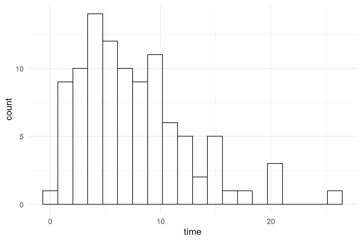
Figure 7.17: Data sampled from a Gamma distribution.
In comparison to the exponential distribution (Figure 7.16), a significant difference is that the mode of the gamma distribution (its peak) is not fixed at zero, but can move along the x-axis. That makes it appear a much more realistic choice for temporal data in behavioral research. We estimate a simple gamma GMM on the simulated data. For historical reasons, brm uses the inverse link function (\(\theta = 1/\mu\)) for Gamma regression per default, but that does not actually serve the purpose of link functions to stretch \(\mu\) into the range of real numbers. Instead, we explicitly demand a log link, which creates a multiplicative model (Table 7.20).
M_gam <- brm(time ~ 1,
  family = Gamma(link = log),
  data = D_gam
)clu(M_gam, mean.func = exp)| parameter | fixef | center | lower | upper |
|---|---|---|---|---|
| b_Intercept | Intercept | 2.03 | 1.90 | 2.17 |
| shape | 2.25 | 1.73 | 2.85 | |
| lp__ | -294.69 | -297.65 | -294.03 |
Both, Exponential and Gamma distributions support the range of real numbers including zero. The weak point of both models is that they have zero as their natural starting point. As we will see in the following section, this assumption is usually violated with RT and ToT data. So, what are they good for, after all? These two models are routinely used for the time intervals (TI) between events that are triggered independently. In nuclear physics the individual triggers are atoms, each one deciding on their own when to decay. If you measure the interval between two decays the time interval is exponentially distributed. (And if you count the neutrons per time interval, the result is a Poisson distribution).
Analog situations can be found in service design and logistics. Take the example of customer support systems. Customers are like atoms in that their decision to file a request is usually independent from each other. Just by chance it can truly happen that two customers call the service center practically in the same moment, so that the lower bound of Zero can actually be reached by some observations. Overwhelmed hotline queues do not make people happy. When planning a support system, the risk of angry customers has to be weighed against the costs of over-staffing. A good design would hit a certain sweet spot and in the ideal case there would be a predictive model of inflow rate of customers.
7.3.2 ExGaussian regression
The problem with RT and ToT data is that Zero is not a possible outcome, as any task uses up a minimum time to complete. For example, Table 7.21 shows the minimum ToT for finding the academic calendar on ten university websites (case Egan). This varies a lot between designs, but is never even close to zero. The last column puts the minimum observed ToT in relation to the observed range. On two of the websites, the offset was even larger than the observed range itself, hence the problem of positive lower boundaries is real in user studies.
attach(Egan)D_egan %>%
filter(
success,
Task == "academic calendar"
) %>%
group_by(Task, Design) %>%
summarize(
min_time = min(ToT),
range = max(ToT) - min_time,
min_time / range
) %>%
arrange(min_time) | Task | Design | min_time | range | min_time/range |
|---|---|---|---|---|
| academic calendar | University of Antwerp | 3 | 7 | 0.429 |
| academic calendar | UGent | 8 | 70 | 0.114 |
| academic calendar | VU Brussel | 21 | 130 | 0.162 |
| academic calendar | UHasselt | 21 | 48 | 0.438 |
| academic calendar | University Tilburg | 24 | 39 | 0.615 |
| academic calendar | KU Leuven | 52 | 40 | 1.300 |
| academic calendar | RUG | 119 | 132 | 0.902 |
| academic calendar | Leiden University | 130 | 181 | 0.718 |
| academic calendar | VU Amsterdam | 207 | 188 | 1.101 |
On the first glance, that does not seem to pose a major problem for Gamma distributions, as the left tail vanishes the more a Gamma distribution is shifted to the right, the impossible regions get smaller. However, Gamma distributions inevitably become more symmetric when moving away from the lower boundary. A Gamma distribution far to the right has almost symmetric tails and we may eventually use a Gaussian distribution for approximation. As there is no separate parameter controlling the skew of the curve it may happen that the random component captures the amount of variance, but overdoes the left tail, which introduces a bias on the coefficients. Figure 7.18 illustrates the mean-variance-skew relationship on three Gamma distributions that move from left to right (M), keeping the variance constant (V):
M <- c(100, 200, 400)
V <- 8000

## gamma
rate <- M / V
shape <- rate^2 * V

ggplot(data.frame(x = c(0, 3000)), aes(x = x)) +
  stat_function(
    fun = dgamma,
    args = list(rate = rate[1], shape = shape[1])
  ) +
  stat_function(
    fun = dgamma,
    args = list(rate = rate[1], shape = shape[2])
  ) +
  stat_function(
    fun = dgamma,
    args = list(rate = rate[1], shape = shape[3])
  ) +
  labs(x = "ToT", y = "density")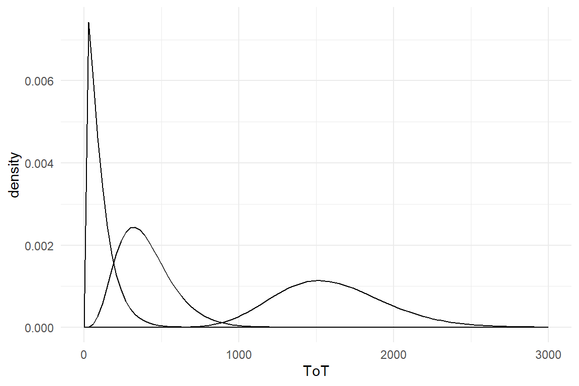
Figure 7.18: Gamma distributions loose their left-skewness, when moving away from the boundary.
So far in this chapter, we have seen that distributions with one parameter (Poisson, binomial, exponential) have a fixed relationship between mean and variance. In order to vary location and dispersion independently, a second parameter is needed (neg-binomial, beta-binomial, Gamma, Gaussian). However, only a three-parameter distributions can do the trick of setting skew separately. So called exponentially modified Gaussian (Exgaussian) distributions are convolutions of a Gaussian distribution and exponential distribution and have three parameters, \(\mu\), \(\sigma\) (as usual) and rate \(\beta\). Very roughly, the Gaussian component controls location and dispersion whereas the exponential part adjusts the skew. When \(\beta\) is large in comparison to \(\mu\), the distribution is more left skewed. With this additional degree of freedom we can simulate (and estimate) distributions that are far to the right, have strong dispersion and strong skew. Figure 7.19 shows Gamma, Gaussian and Exgaussian distributions with exact same mean and variance.
M <- 400
V <- 8000

## Exgaussian
mu <- M
beta <- 80
sigma <- sqrt(V - beta^2)

## Gamma
rate <- M / V
shape <- rate^2 * V

ggplot(data.frame(x = c(0, 800)), aes(x = x)) +
  stat_function(
    fun = dgamma,
    args = list(rate = rate, shape = shape),
    mapping = aes(colour = "Gamma")
  ) +
  stat_function(
    fun = dnorm,
    args = list(mean = M, sd = sqrt(V)),
    mapping = aes(colour = "Gaussian")
  ) +
  stat_function(
    fun = brms::dexgaussian,
    args = list(
      mu = M,
      sigma = sigma,
      beta = beta
    ),
    mapping = aes(colour = "Exgaussian")
  ) +
  labs(colour = "Distribution", x = "ToT", y = "density")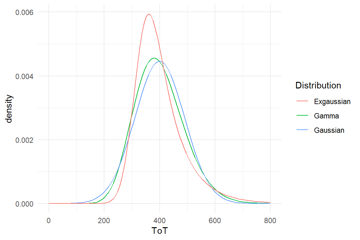
Figure 7.19: Exgaussian distributions can be far from zero and still be left skewed
The Gamma distribution in this example starts approaching a the perfect bell curve of the Gaussian distribution. In contrast, the Exgaussian distribution takes a steep left climb followed by a long right tail, which is caused by its pronounced exponential component. We do the usual exercise to simulate a grand mean model (Figure 7.20) and recover the parameters with the help of the brm engine (Table 7.22))
attach(Chapter_GLM)set.seed(126)
D_exg <-
tibble(Y = rexgaussian(100, mu = 100, sigma = 20, beta = 30))
qplot(D_exg$Y) + xlim(0, 300)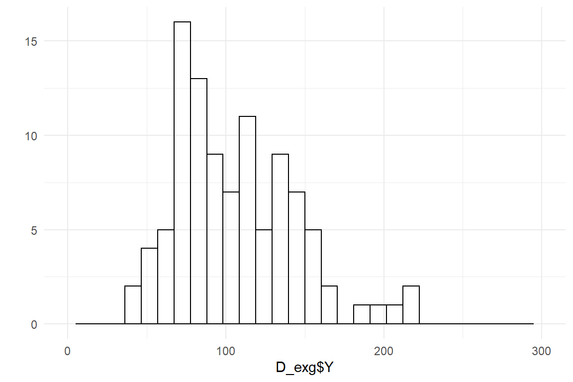
Figure 7.20: Sampling from an Exgaussian distribution
M_exg <- brm(Y ~ 1,
  family = exgaussian,
  data = D_exg
)clu(M_exg)| parameter | fixef | center | lower | upper |
|---|---|---|---|---|
| b_Intercept | Intercept | 99.4 | 92.9 | 106.6 |
| sigma | 17.7 | 12.3 | 24.0 | |
| beta | 31.6 | 23.5 | 41.6 | |
| lp__ | -500.1 | -503.6 | -499.0 |
Noteworthy, for Exgaussian models the brm engine uses the identity link function by default. While this is rather convenient for interpretation, it could theoretically lead to impossible predictions. As we will see later, the Exgaussian family is not immune, but robust to impossible predictions because of its tiny left tail.
Most GLM family members introduced so far are more or less established in the literature. The Exgaussian is a newcomer and it does not come with a clear cut data generation process and may therefore very well be considered just a hack. The following two sections examine Exgaussian models more closely and out them in competition against Gamma and Gaussian models. We will be using primarily graphical methods here, but will come back these cases in chapter 8.2.5 with a more formal approach.
7.3.2.1 Reaction times
In experimental studies, the inertia of the nervous system sets a limit larger than zero for reaction times. This is partly due to to some hard electrochemical and biomechanical limits of the peripheral systems. (Perhaps, octopuses with their long arms have decentralized nervous system for a reason!) Nerve cells and muscle fibers are slow working horses, adding to the time our minds need to process complex information. Even in the most simple priming experiments, there always is a minimum time necessary to collect an idea from the memories and activate the surrounding nodes. Therefore, experimental reaction times have a positive minimum of at least 200ms.
Let’s see an example: In the Hugme case, we tried to pin down the hypothetical Geek personality and used Need-for-cognition as a predictor for reaction times in a semantic Stroop task. Like in the original Stroop task, participants must name the color of words, but these are non-color words from two categories (geek/non-geek). Furthermore, these words are preceded by Geek/non-geek pictures. The theory was that a real geek, when seeing an open computer case followed by the word “explore” will briefly reminisce and be distracted from the primary task, naming the color. It did not work this way at all and we only saw minuscule effects. That is good news for the analysis here. The only effect was that Geek primes caused a minimal delay. Because there are no other effects, we can use a rather simple multi-level CGM to compare how Gaussian, Gamma and Exgaussian fit reaction times. Let’s take a first look some parts of the data:
attach(Hugme)Most of the participant-level frequency distributions of RT have a clear cut-off at around .25 seconds. The steepness of the left climb varies between participants, but some at least are rather sharp, with a right tail that is leveling off slowly. When compared to the illustrations above, it seems that an Exgaussian model could accommodate this data well (Figure 7.21).
D_hugme %>%
  filter(Part <= 6) %>%
  ggplot(aes(y = RT, x = PrimeGeek)) +
  facet_wrap(~Part, nrow = 2) +
  geom_violin()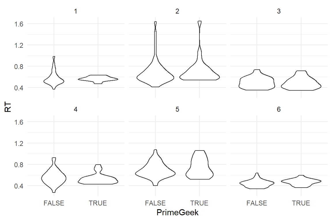
Figure 7.21: Participant-level RT distributions
Even the effect of geek primes is barely visible, but we clearly observe a left skew in most of the participants. In the following, we run three CGM models with Exgaussian, Gamma or Gaussian response distributions. For the subsequent analysis, multi-model posterior distributions and posterior predictive distributions are extracted and merged into one multi-model posterior object P_1.
memory.limit(16000)

F_1 <- formula(RT ~ 1 + PrimeGeek + (1 + PrimeGeek | Part))

M_1_gau <- D_hugme %>%
  brm(F_1,
    family = gaussian,
    data = .
  )

M_1_gam <- D_hugme %>%
  brm(F_1,
    family = Gamma(link = identity),
    data = .
  )

M_1_exg <- D_hugme %>%
  brm(F_1,
    family = exgaussian,
    data = .
  )

P_1 <- bind_rows(
  posterior(M_1_gau),
  posterior(M_1_gam),
  posterior(M_1_exg)
)

T_1_predict <-
  bind_rows(
    post_pred(M_1_gau, thin = 5),
    post_pred(M_1_gam, thin = 5),
    post_pred(M_1_exg, thin = 5)
  ) %>%
  predict()
Note that the predictive posterior distributions runs over thousands of observation, which creates very large objects in your computer’s RAM. To prevent running into a memory limit, you can crank up the memory limit (memory.limit) or thin out the number of posterior predictive samples by a factor, or do both.
The below plot shows the population-level effects for the three models. The center estimates are very close, which means that neither of the models has a significant bias. However, the Exgaussian model produces much tighter credibility intervals. We have seen such an effect before, when on over-dispersed data, a Poisson model produced tighter intervals than the Negbinomial model. Here it is the other way round: the model with more parameters produces better levels of certainty (Figure 7.22).
fixef(P_1) %>%
  ggplot(aes(
    y = center, ymin = lower, ymax = upper,
    x = model
  )) +
  facet_wrap(~fixef, scales = "free") +
  geom_crossbar(width = .2, position = "dodge")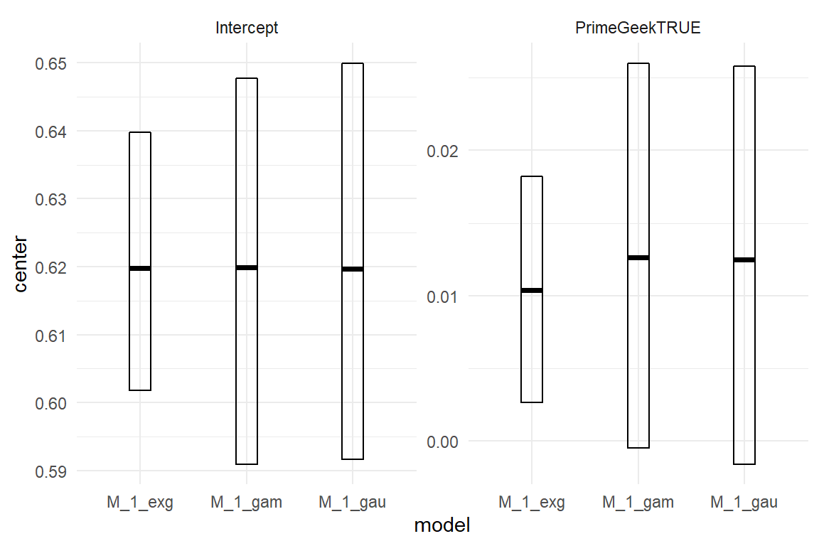
Figure 7.22: Comparing CLU estimates of Exgaussian, Gamma and Gaussian models
If the Exgaussian model has a better fit, we should primarily see that in how the residuals are shaped. The Exgaussian distribution has one more degree of freedom, which can be used to set an arbitrary skew. The following reveals that the extra flexibility of the Exgaussian has been employed. Both, Gaussian and Gamma are almost symmetric, whereas the Exgaussian takes a steeper left climb. The three distributions have almost the same right tail, but the left tail of the Exgaussian is consistently shorter.
D_hugme <- D_hugme %>%
  left_join(T_1_predict) %>%
  mutate(resid = RT - center)

D_hugme %>%
  ggplot(aes(y = resid, x = PrimeGeek)) +
  facet_grid(. ~ model) +
  geom_violin()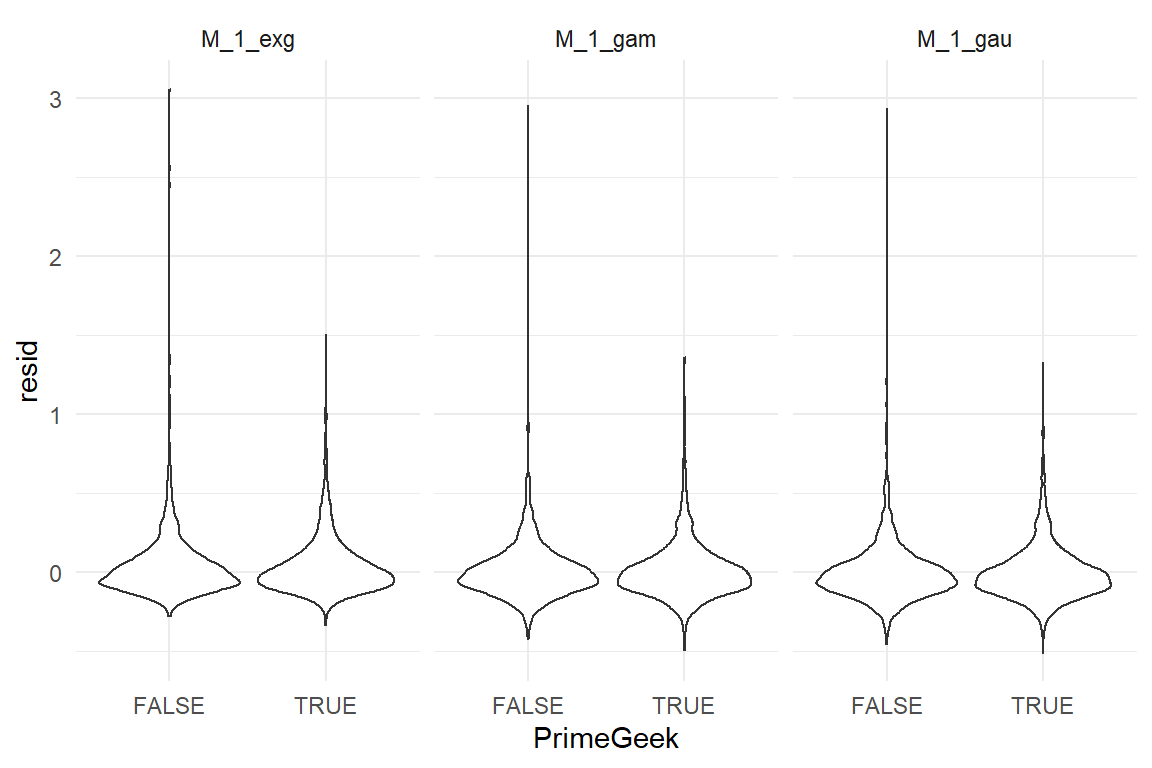
Figure 7.23: Comparing residuals of Exgaussian, Gamma and Gaussian models
We can carefully conclude that the Exgaussian may be very useful for analyzing psychological experiments as it seems to better accommodate reaction times. Given the novelty of Exgaussian models, it is recommended that researchers carry out a careful multi-model analysis. In 8.2.5 we will come back to this case with a more formal approach and confirm that from the three response distributions, the Exgaussian has the best predictive accuracy.
7.3.2.2 Time-on-task
Experimental psychologists call the Stroop task a complex one. But, essentially it is a decision between three colors and minimal processing time is rather short. Compared to tasks in usability studies, such as finding information on websites, this is almost trivial. Also, the dynamics of complex tasks can be rather different. For example, a single user error at the beginning of a task sequence can have dramatic consequences, such as getting totally lost. While ToT data also has a strictly positive lower boundary (the fastest way of achieving the goal), it often has a much wider spread than RT data. In the following we will repeat the informal model comparison from the last section for ToT data.
We compare the three patterns of randomness on the CUE8 data set, which contains ToT measures on five tasks on a car rental website. In this study 14 professional teams took part with two conditions: remote and moderated sessions. As data from the remote condition is contaminated with cheaters, we only use the moderated sessions. In order to compare the impact of the chosen distribution on the coefficient estimates, we examine the estimation of the five tasks (as an AGM).
attach(CUE8)D_cue8_mod <-
D_cue8 %>%
filter(Condition == "moderated", !is.na(ToT)) %>%
as_tbl_obs()F_4 <- formula(ToT ~ 0 + Task + (1 | Part))
M_4_gau <- D_cue8_mod %>%
brm(F_4,
family = gaussian(link = log),
data = ., iter = 2000
)
M_4_exg <- D_cue8_mod %>%
brm(F_4,
family = exgaussian(link = log),
data = ., iter = 2000
)
M_4_gam <- D_cue8_mod %>%
brm(F_4,
family = Gamma(link = log),
data = ., iter = 2000
)
P_4 <- bind_rows(
posterior(M_4_gau),
posterior(M_4_gam) %>% mutate(value = if_else(value %in% c("fixef", "ranef"), exp(value), value)),
posterior(M_4_exg)
)
T_4_predict <- bind_rows(
post_pred(M_4_gau, thin = 5),
post_pred(M_4_gam, thin = 5),
post_pred(M_4_exg, thin = 5)
) %>%
predict()Note that the Gamma model caused trouble when estimated with an identity link. For this reason, all three models were estimated on a log-linearized scale. This makes the back-transformed coefficients multiplicative, which actually makes more sense, as we have seen in 7.2.1.1.
fixef(P_4, mean.func = exp) %>%
  ggplot(aes(
    y = center, ymin = lower, ymax = upper,
    x = model
  )) +
  facet_wrap(~fixef) +
  geom_crossbar(width = .2) +
  theme(axis.text.x = element_text(angle = 45, hjust = 1))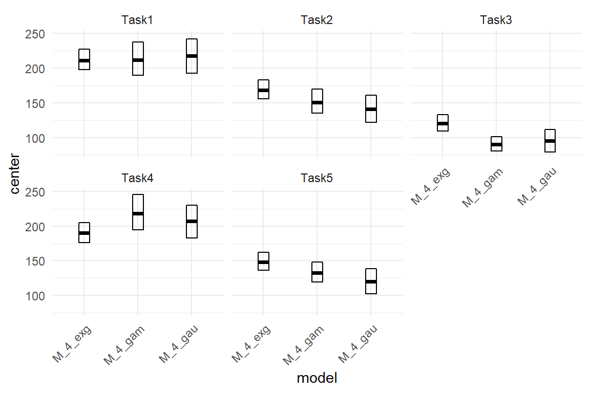
Figure 7.24: Comparing CLU estimates of Exgaussian, Gamma and Gaussian models
In the previous section 7.3.2.1, we have seen for RT data, that the three models agreed on the center estimates. As shown in Figure 7.24, for ToT data the three families produce rather different coefficients. It seems that the models disagree on all but Task 1. It is not more than an observation, but the Exgaussian model produces the smallest variance between tasks. A recurring observation is that Exgaussian regression also produced the tightest credibility intervals.
Inspecting the residual distributions yields a similar pattern as with RT data: the Exgaussian model predicts a much sharper left raise than the other two.
left_join(T_4_predict, D_cue8_mod, by = "Obs") %>%
  mutate(resid = ToT - center) %>%
  ggplot(aes(x = model, y = resid)) +
  facet_wrap(~Task, nrow = 2) +
  geom_violin() +
  theme(axis.text.x = element_text(angle = 45, hjust = 1))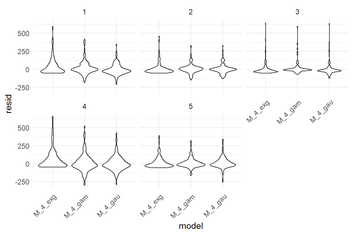
Figure 7.25: Comparing residuals of Exgaussian, Gamma and Gaussian models
In general, it seems that Exgaussian models for RT and ToT accommodates left skew better and produces estimates that are sharp and conservative. But, These are just informal comparisons. In chapter 8, we will apply formal criteria for selecting between distributions. As will turn out, Gamma distribution is the preferred distribution for ToT in CUE8.
One last issue remains to get clarified: using the identity link for Exgaussian models is very convenient and is probably much safer as compared to Gaussian models with their fatter left tails. Still, impossible predictions can arise. But, how much of a risk is there? We can check this on the posterior predictive distributions of both studies, CUE8 and Hugme. Table 7.23 shows the proportion of observations, that get a negative 2.5% credibility limit assigned.
bind_rows(Hugme$T_1_predict, CUE8$T_4_predict) %>%
  group_by(model) %>%
summarize(mean(lower < 0)) | model | mean(lower < 0) |
|---|---|
| M_1_exg | 0.000 |
| M_1_gam | 0.000 |
| M_1_gau | 0.000 |
| M_4_exg | 0.014 |
| M_4_gam | 0.000 |
| M_4_gau | 0.750 |
For the RT data (M_1), impossible predictions are not an issue with any of the models, as all 2.5% quantiles are positive. That is different for ToT (M_4): while the Gamma model is inherently immune to negative predictions, the Exgaussian model produced a few impossible lower 2.5% limits (around 3%). The Gaussian model is extremely off: more than 70% of all predictions have impossible lower 2.5% limits.
In the scientific literature, using the Gaussian model for RT and ToT is still the default. Probably, that is due to the lack of user-friendly engines supporting the more exotic GLM family members, Gamma or Exgaussian regression. The Brms engine covers a much broader set of distributions than any other implementation before and researchers have the choice. This chapter attempted to provide theoretical arguments as well as empirical indications that the Exgaussian regression can be a better choice than Gaussian and gamma. First of all, it accommodates the strong left skew of RT and ToT much better than the Gamma, which takes a too symmetric form when far from the left boundary. Second, it is reasonably robust to impossible predictions, even when using the convenient identity link function. Third, and that is almost too good to be true, it strongly improves certainty in predictors. It seems that Exgaussian models are more efficient for carving out delicate effects in experimental studies.
However, as the discussion has just started, to declare it settled would be premature. In contrast, the aim of this section was to illustrate a semi-formal approach that researchers can follow to choose among the candidate models for their specific RT and ToT data. Data from other RT paradigms might take different shapes. For example, when measuring RT by events in EEG signals (rather than actual key presses), motor time plays a much smaller role, pushing RTs closer to the left boundary and the Gamma model would be in favor.
That being said, the brms engine offers even more opportunities. First, it supports two more distributions with an offset component: the shifted log-normal and the Wiener distribution. Interestingly, the latter grounds on one of the few formally specified cognitive process models, the diffusion model for simple choice tasks. All four parameters of the Wiener distribution are directly linked to individual elements of the cognitive process. This brings us to another extension of Brms, which I will briefly cover in the last section of this chapter. Distributional models put linearized predictor terms not just on the distribution mean, but also on other parameters of a distribution family. It is thrilling to imagine what such models can do for experimental cognitive research.
7.4 Rating scales
In classic design research of the last millennium, die-hard Human Factors researchers have mainly been asking objectively sounding questions, like:
- Can a user achieve accurate results with the system?
- Can they do so in less time?
- Is the number of errors reasonably confined?
For professional systems, these are still highly valid questions. For example, the purpose of a medical infusion pump is to improve the health status of a patient by accurately and reliably delivering medication into the bloodstream and the extent to which a nurse achieves this by correctly programming the device can be measured directly.
However, starting with the 1990s, wave after wave of novel electronic entertainment systems and digital gadgets rolled over the consumer market and user feelings got more into the focus. The purpose of a video recorder or a smartphone is to deliver joy. With the new millennium, design researchers began to recognize what consumer psychologists had discovered two decades earlier: users are not rational decision makers in a utilitarian sense, but are lead by their feelings. When people decide to adopt (or buy) a new system, this is only partly driven by their expectation of productivity. Such feelings come as a variety of different constructs:
- feeling of joy
- expression of self
- social connectedness
- aesthetic perception
- personal growth
Whether or not these concepts are well-defined from a psychological point-of-view is beyond the scope of this book. What matters is that feelings are so elusive, that the most sincere researchers have not yet found objective criteria to measure them. Instead, almost everyone resorts to use of self-report rating scales, like this one:
How beautiful do you perceive the user interface to be?
unattractive 1 – 2 – 3 – 4 – 5 a piece of art
If you use a 5 point rating scale like this one to measure perceived beauty, it is the participants who convert their gut feeling into a number. This is a hidden and uncontrolled process, but it presumably involves the following three subprocesses:
- anchoring
- introspection
- binning
By anchoring participants establish an idea of how ugly or beautiful something has be to get an extreme rating of 1 or 5. These imaginary endpoints define the absolute range of the rating scale. The researcher might early on give explicit or implicit cues to let the participant guess the class of to-be-rated objects. If an experiment is overtly about web design, then probably “very ugly” means the least attractive commercial website the participant can think of. However, participants old enough to remember web design in its infancy (say the early attempts of disney.com), may end up with a lower anchor than today’s kids. If not enough cues are given upfront, participants will make up their own minds (in an uncontrolled way) and at best adjust their anchors to the stimuli they see throughout the experiment. Probably, it will make a difference for what 1 or 5 mean, when the set of stimuli contain just websites, or websites and impressionist paintings and horrifying screenshots from splatter movies or brutal computer games.
By introspection participants intuitively assess the intensity of their real feelings as compared to the anchors. Reportedly, such feelings are influenced by:
- visual simplicity
- prototypicality
- second exposure
- Gestalt principles
- fluency of processing
- attribute substitution heuristics
- color aesthetics
- fashion
- previous stimuli
- current mood
- a person’s history
- and cultural background
Finally, by binning the participant mentally divides the absolute range into five categories that are either fuzzy or defined by stereotypes, like “It must look at least as elegant as the Mapple website to get a 4.”
As the outcome of anchoring, introspection and binning are not under the control of the researcher, the response patterns can vary between participants. Let’s consider a few possible patterns of participants (and their dramatic stories, see Figure 7.26):
- A is indecisive and stays in the center region
- B has a crush on the experimenter and always responds slightly more positive
- C is Swedish and avoids extremes
- D is a civil rights activist and habitually treats all bins equally.
- E is annoyed by the experiment and falls into an almost dichotomous pattern
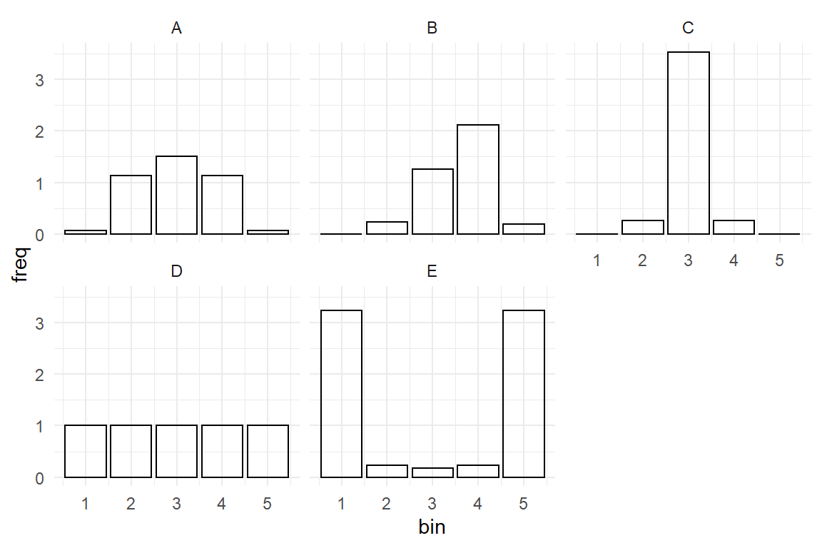
Figure 7.26: Five participants with different response styles
Many unknowns are in the game. Only one special case we can alleviate with the multilevel modeling tools in our hands. Anchoring can (but not necessarily does) result in a constant shift between participants. Compare participants A and B: A collects almost all stimuli in categories 2, 3 and 4, whereas B uses 3, 4 and 5. This is not much else than a participant-level intercept random effect. Unfortunately, the situation can be more difficult than that. When participants differ in how extreme they set their endpoints, like C and D, their responses will differ in variance. The maximum variance, however, will be found in participant D.
To speak of a real case: In the IPump study, a single-item rating scale was used to measure mental workload. The results suggest that all participants used the lower range of the scale, but differed vastly in where they set their upper point. Figure 7.27 orders participants by the maximum value they used. This is obviously related to variance, but seemingly not so much with location. It does not suffice to use a response distribution with mean-variance relationship, as we used to. All these issues make rating scales peculiar and we should not pretend they have the same neat arithmetic properties as objective measures.
attach(IPump)

D_pumps %>%
  group_by(Part) %>%
  summarize(
    min = min(workload),
    max = max(workload),
    median = median(workload)
  ) %>%
  mutate(Part_ord = rank(max, ties.method = "first")) %>%
  ggplot(aes(x = Part_ord, ymax = max, ymin = min, y = median)) +
  geom_crossbar() +
  labs(x = "Part(ordered)", y = "workload")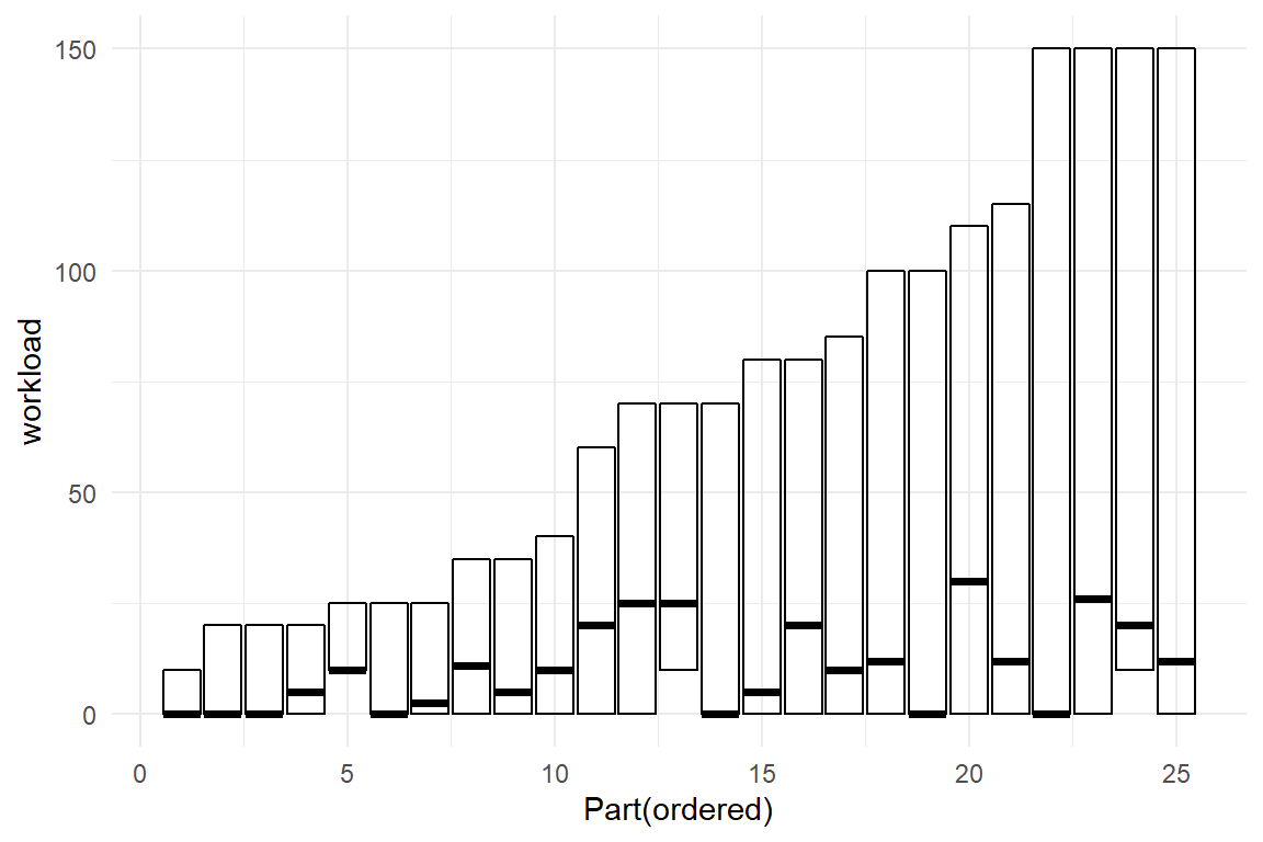
Figure 7.27: In the IPump study participants vary greatly in how they exploit the range of a mental workload scale.
Setting the idiosyncratic rating scale responses aside, how does a common rating scale appear in our framework of link functions and patterns of randomness? Rating scales are bounded on two sides and we already know what that means: a suitable model for rating scales will likely contain a logit link function and a distribution of randomness that is bounded on two sides.
A real problem with rating scales is that they often are discrete. Most instruments force participants to give their answer as a choice between five or seven ordered levels. When the response variable has just a few levels, ordinal regression is a good choice, which is an extension of logistic regression.
However, most properly designed rating scales are composed of several items, because only that can sufficiently reduce measurement error and allow for in-depth psychometric assessments (6.8). While from a psychometric perspective, single-item scales are susceptible, there can be situations where a researcher may use a validated single item scale for pragmatic reasons. Especially, when measures happen in-situ, such as during a usability test or even a real operation, being brief and unobtrusive might be more important than perfecting the measures.
With multi-item rating scales, one also has the possibility to build a psychometric multi-level model, where items are considered a sample of a population of possible items. That is actually a very good idea, as the item-level random effects control for differences in item location. For example, the following item is likely to produce generally lower beauty ratings than the one shown earlier, because the anchors have been moved downwards:
How beautiful do you perceive the user interface?
like a screenshot from a splatter movie 1 – 2 – 3 – 4 – 5 quite attractive
Unless one builds such a psychometric multi-level model, ordinal regression is not very suitable for multi-item scales and here is why: The sum (or mean) score is still binned, but more finely grained. A sum score over three seven-binned items already has 21 bins, which would result in an inflation of number of parameters in ordinal regression.
As a rescue, one might well regard a measure with 21 bins as continuous . Furthermore, there actually is no strong reason to use binned rating scales at all. So called visual analog scales let participants make continuous choices by either drawing a cross on a line or move a slider control. For sum scores and visual analogue scales, the problem of choice reduces to a logit link function (they still have two boundaries) and a continuous distribution bounded on both sides. That is precisely what is behind beta regression and, as we shall see, this distribution is flexible enough to smooth over several of the rating scale problems that were just discussed.
7.4.1 Ordered logistic regression
When the ordinal response has a low number of response categories (between 4 and 7), ordinal regression applies. Recall logistic regression: the response falls into one of two categories, which are coded as 0 and 1. Although not in a strict sense, the two categories can often be thought of as in an order: success is better than failure, presence more than absence and a return better than staying away. Instead of two categories, we can also conceive the situation as a threshold between the categories, that needs force to jump over it. Any positive impact factor \(x_i\) can then be thought of as such a force that pushes a response probability to the higher category, by the amount \(\beta_i\) (on logit scale). At the same time, the intercept \(\beta_0\) represents the basic log-odds of falling into category 1 in a default state, that is \(x_i = 0\).
In ordinal regression, the idea of thresholds is extended more than two ordered response categories. The only arising complication is that with two categories, we have one threshold to overcome, whereas with three categories there are two thresholds and generally, with \(c\) categories, there are \(c - 1\) thresholds. Ordinal regression deals with the problem by estimating \(c - 1\) intercept estimates \(\beta_{0[k]}\). Each threshold intercept \(\beta_{0[k]}\) represents the probability (on logit scale) that the response falls into category \(k\) or lower, or formally:
\[ \text{logit}(P(y_i \leq k)) = \beta_{0[k]} \]
Let’s see this at the example of the BrowsingAB case, first. User ratings have been simulated with seven levels (Figure 7.28):
attach(BrowsingAB)BAB1 %>%
ggplot(aes(x = rating)) +
facet_grid(Design ~ .) +
geom_histogram() +
xlim(1, 7)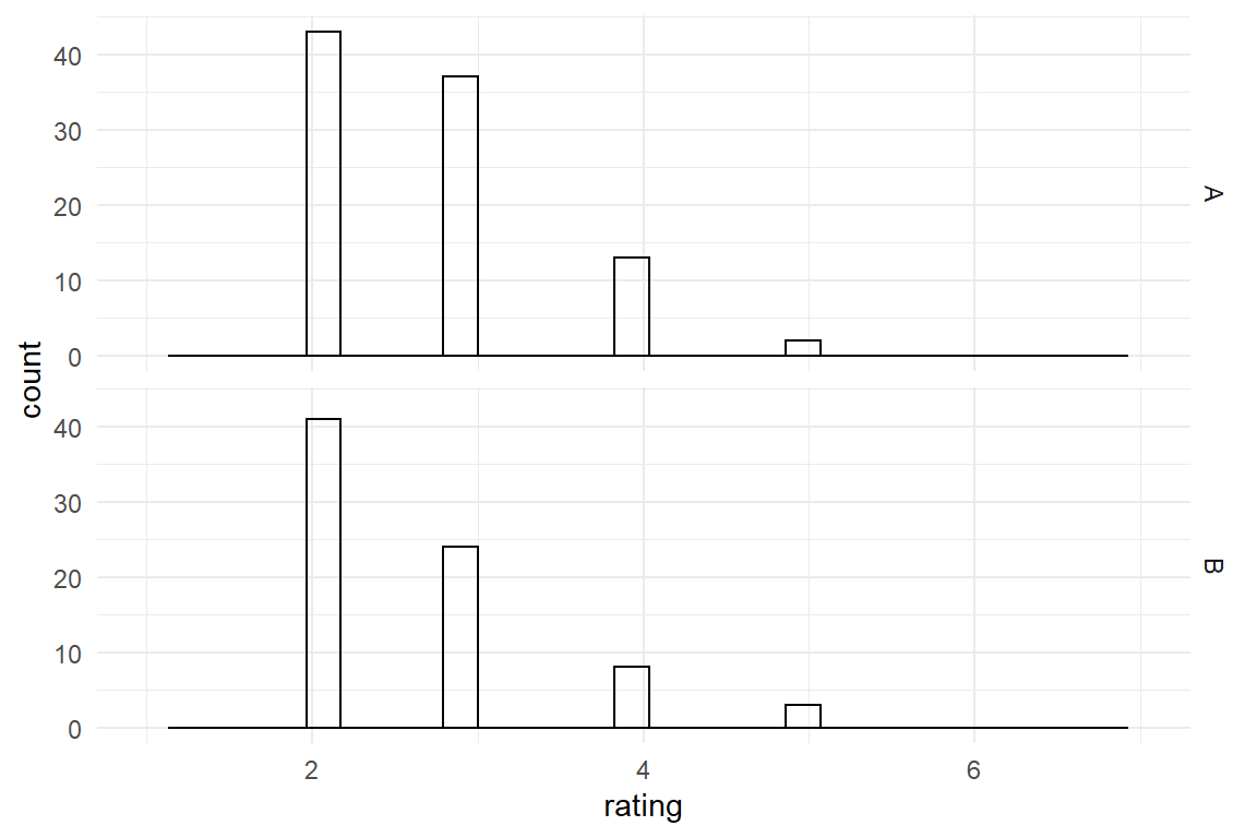
Figure 7.28: Designs A and B rated on a sevel-point scale
The brms regression engine implements ordinal regression by the family cratio (cumulative odds ratio ) with a default logit link function.
M_ord_1 <-
  BAB1 %>%
  brm(rating ~ Design,
    family = "cratio",
    data = .
)fixef(M_ord_1)| fixef | center | lower | upper |
|---|---|---|---|
| -2.072 | -2.557 | -1.607 | |
| -0.276 | -0.633 | 0.075 | |
| 0.646 | 0.168 | 1.162 | |
| 1.205 | 0.320 | 2.274 | |
| DesignB | -0.543 | -0.955 | -0.122 |
The six intercepts correspond with the thresholds between the seven levels. It is no coincidence that the intercept estimates increase by order, as they are cumulative (the “c” in cratio). The first intercept estimate represents (the logit of) the proportion of responses \(y_i \leq 1\), the second \(y_i \leq 2\) etc. The Design effect has the usual interpretation as compared to logistic regression, a change in odds. The only difference is that it now acts on all six reference points. The expected proportion of responses equal to or smaller than 2 for design A is:
\[ \begin{aligned} \pi(y_i \leq 2|A) &= \text{logit}^{-1}(\beta_{0[2]}) \\ &=\text{logit}^{-1}(-0.3) = 0.426 \end{aligned} \]
The expected proportion of responses equal to or smaller than 2 for design B we get by the usual linear combination:
\[ \begin{aligned} \pi(y_i \leq 2|B) &= \text{logit}^{-1}(\beta_{0[2]} + \beta_1) \\ &= \text{logit}^{-1}(NA) = NA \end{aligned} \]
All coefficients are shifting all thresholds by the same amount (on the linear predictor scale). You can picture this as a single puppeteer controlling multiple puppets by just one stick, making them dance synchronously. As long as the ordinal scale has only a low number of bins, that keeps the number of parameters at a reasonable level. Just imagine, you were estimating an ordinal multilevel model and all participant-level effects were five or seven-folded, too. However, the equidistancy of effects on bin thresholds is an assumption by itself, and in the presence of response styles on rating scales, it cannot be taken for granted .
Besides that, the ordinal model appears very snug to the structure of the data. It does not wipe over the fact that the response is discrete and the thresholds represent the order. Conveniently, effects are represented by a single estimate, which one can use to communicate direction and certainty of effects. On the downside, communicating absolute performance (that is, including the intercept) is more complicated. When presenting predictions from an ordinal model one actually has to present all thresholds, rather than a single mean. In practice that probably is less relevant than one might think at first, because predictions on self-report scales is less useful than metric performance data. Ordinal data also does not lend itself so much to further calculations. For example, you can use ToT measures on infusion pumps in calculating the required staffing of an intensive care unit, because seconds are metric and can be summed and divided. In contrast, it does not make sense to calculate the cognitive workload of a team of nurses by summing their self-report scores. The only possibility is to compare the strengths of predictors, but that does not require predictions.
7.4.2 Beta regression
In my opinion, one of the most futile discussions in methodology research whether one should use a four, five or seven binned Likert scale. From a pure measurement point of view, more bins give better resolution, the ultimate consequence being not to bin at all, that is using continuous rating scales. At the same time, many rating responses come from multiple item scales, which multiplies the number of bins. Speaking of ordinal regression, it seems reasonable to have seven intercepts for a single item scale, but who would want 14 or 21 for a two or three-item scale? And most scales have even more items.
Psychometric research in the process of developing rating scales routinely uses a method called confirmatory factor analysis, which derives from the Gaussian linear model and inherits its assumptions. As always, Gaussian models are sometimes a reasonable approximation, but given the framework of GLM, it is unnecessary (to put it mildly) to go along with the Gaussian, violating the assumptions of normality and linearity. While the link function for a double bounded response variable is simply the logit, the only missing ingredient is a double bounded error distribution. Enter Beta distribution!
We demonstrate beta regression on rating scales at the example of the CUE8 study. This study aimed at assessing whether remote usability testing arrives at the same ToT measures as in moderated sessions. As we have seen in 6.6, the difference is marginal for ToT.
As rating scales are susceptible to all kinds of cognitive and social biases, a golden rule for user test moderators is to constantly remind participants to not blame themselves for errors. Reportedly, test moderators also do help participants (after counting to 10) in order to minimize frustration (and maximize information flow). What could the presence or absence of a moderator do to satisfaction ratings? Perhaps, remote participants feel the lack of assurance and support as higher levels of frustration. Furthermore, it is not unlikely that satisfaction ratings are sensitive to idiosyncrasies in the process of the user test, such that we could even expect differences between teams.
Before we build the model, there are two issues to regard: First, the boundaries of Beta distributions are 0 and 1, which requires a rescaling of responses into this interval. The SUS scores are on a scale from 0 to 100 and a divisor of 100 would produce the desired interval. Second, the responses must actually lie strictly between 0 and 1, excluding the boundaries. On (quasi)continuous scales, it seems not very likely to have 0 or 1 as response, but it can happen. Indeed, participants in the CUE8 study have responded with a satisfaction rating of 100 quite often.
A practical solution is to scale the responses in such a way as to avoid the two boundaries, which is what the following hack does.
- add a tiny value to all responses
- create a divisor by adding twice that value to the maximum value the responses can take
- divide all responses by that divisor
You may find it inappropriate to mangle a response variable in such an arbitrary way. However, keep in mind that the levels of ordinal responses are highly arbitrary. In terms of measurement theory, all transformations that maintain the order are permitted for ordinal scales. For the following analysis, the data set was further reduced by averaging the scores across tasks and excluding probable cheaters with a ToT < 30s.
attach(CUE8)D_cue8_SUS <-
D_cue8 %>%
filter(!is.na(SUS)) %>%
group_by(Part, Team, Condition) %>%
dplyr::summarize(
ToT = sum(ToT),
SUS = mean(SUS)
) %>%
ungroup() %>%
filter(ToT > 30) %>%
mutate(SUS = mascutils::rescale_unit(SUS)) %>%
as_tbl_obs()
D_cue8_SUS %>%
ggplot(aes(x = Team, y = SUS)) +
facet_grid(~Condition) +
geom_violin() +
geom_count()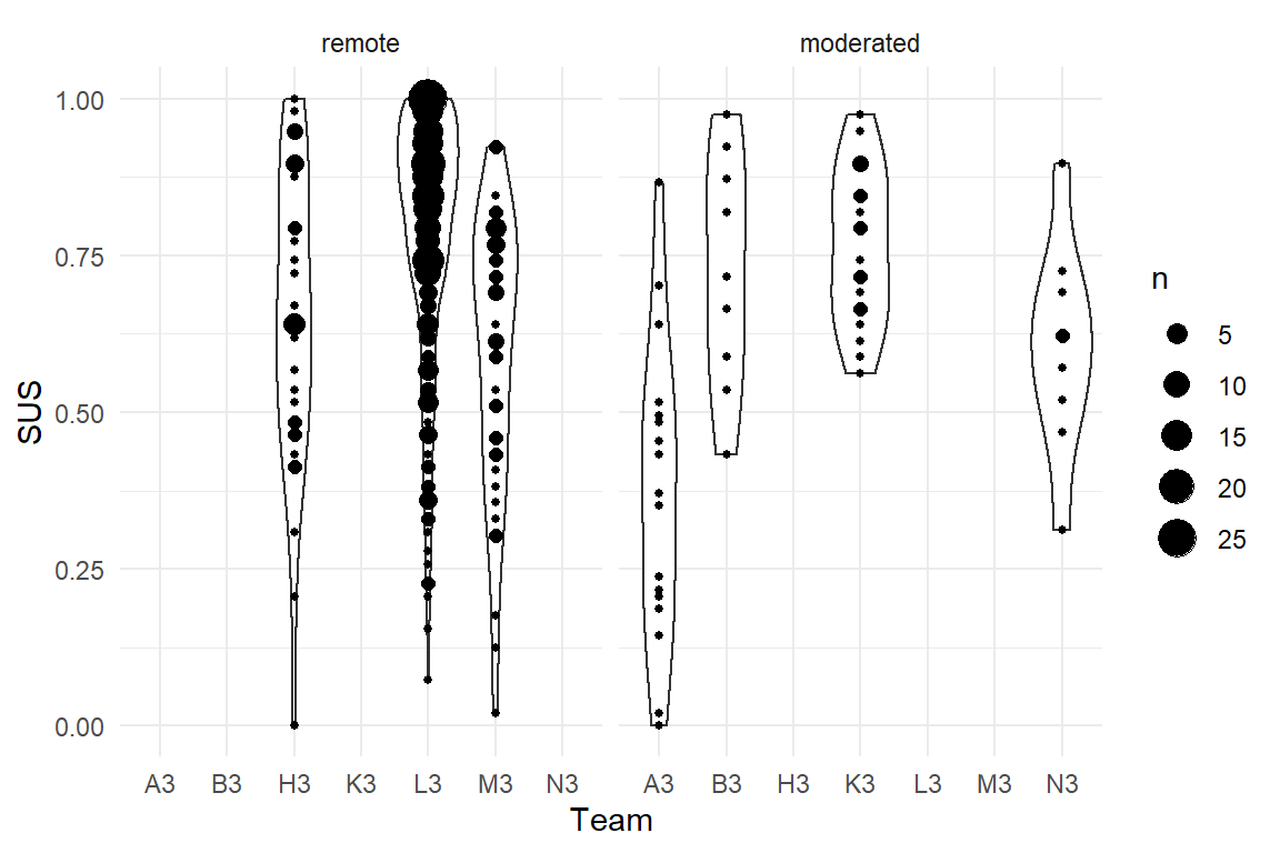
Figure 7.29: Response distribution of SUS ratings across teams and conditions
M_5_bet <-
  D_cue8_SUS %>%
  brm(SUS ~ Condition + (1 | Team),
    family = Beta(link = "logit"),
    data = .
)fixef_ml(M_5_bet)| fixef | center | lower | upper | SD_Team |
|---|---|---|---|---|
| Intercept | 0.771 | -0.131 | 1.645 | 0.678 |
| Conditionmoderated | -0.300 | -1.572 | 0.958 |
Do participants in remote sessions feel less satisfied? There seems to be a slight disadvantage, but we cannot confirm this with sufficient certainty. In contrast, the variation between teams is substantial, which indicates that SUS ratings are not independent of the particular setting. That is rather concerning for a widely used and allegedly validated rating scale.
7.5 Beyond mean: distributional models
The framework of GLM, as flexible as it has proven to be up to this point, has one major limitation: it only renders the relationship between predictors and the mean of the distribution. We only think in terms of impact factors that improve (or damage) average response times, error rates, satisfaction ratings etc. As we have seen multiple times in chapter 6, variance matters, too. With multi-level models we can estimate variance within a sample and even compare variance across samples, like in the CUE8 case, where more variance is due to teams rather than due to participants.
What cannot be done with plain multi-level models is estimate effects on variance, like: “Do teams in CUE8 differ in the variation of responses?” That brings me to the final feature of modern regression modeling in the scope of this book. With distributional models, we can put predictors on any distribution parameter that we want, not just location \(\mu\).
All but the one-parameter distributions come with additional parameters that allow to accommodate the dispersion of the error distribution, or even its skew in the case of Exgaussian models. In the following I will present two application scenarios for distributional models. We start with a designometric problem when using bi-polar rating scales (see 7.4.) In the next section I will illustrate the problem on simulated data from two items with different anchoring. Subsequently, we will see on a real data set, that participants differ in how they exploit the range of a rating scale. by a simple simulation will show what effect item anchoring can have and how a distributional model can deal with such a situation.
7.5.1 Item-level anchoring in rating scales
As a first illustration, imagine two versions of a continuous rating scale for visual beauty that differ in how their anchors are labeled. The first question is moderately labeled, the second is extreme.
- like the ugliest website I have ever seen: 0 ——– 1 like the most beautiful website
- distgusting as a screenshot from a splatter movie: 0 ——– 1 like the most beautiful impressionist painting
For the sake of simplicity (not for a strong research design), let us assume that one participant has rated a sample of 400 websites in two conditions: moderate anchoring and extreme anchoring. The following simulates data such that both anchorings have the same location (mu), but the moderate anchoring condition produces a much more exploitation of the range. Note that Beta distribution’s parameter phi does not increase variance, but just the opposite: the range of the scale is expanded, which lets the variance shrink. It is comparable to the number of trials in a binomial process. The more trials there are, the relatively tighter the distribution becomes (Figure 7.30)
set.seed(42)

N <- 400

Conditions <-
  tribble(
    ~Anchoring, ~mu, ~phi,
    "extreme", .3, 18,
    "moderate", .3, 6
  ) %>%
  mutate(
    a = mu * phi,
    b = phi - mu * phi
  )

D_Anchor <-
  tibble(
    Obs = 1:N,
    Anchoring = rep(c("extreme", "moderate"), N / 2)
  ) %>%
  left_join(Conditions) %>%
  mutate(rating = rbeta(N, a, b))

D_Anchor %>%
  ggplot(aes(x = Anchoring, y = rating)) +
  geom_violin() +
  ylim(0, 1)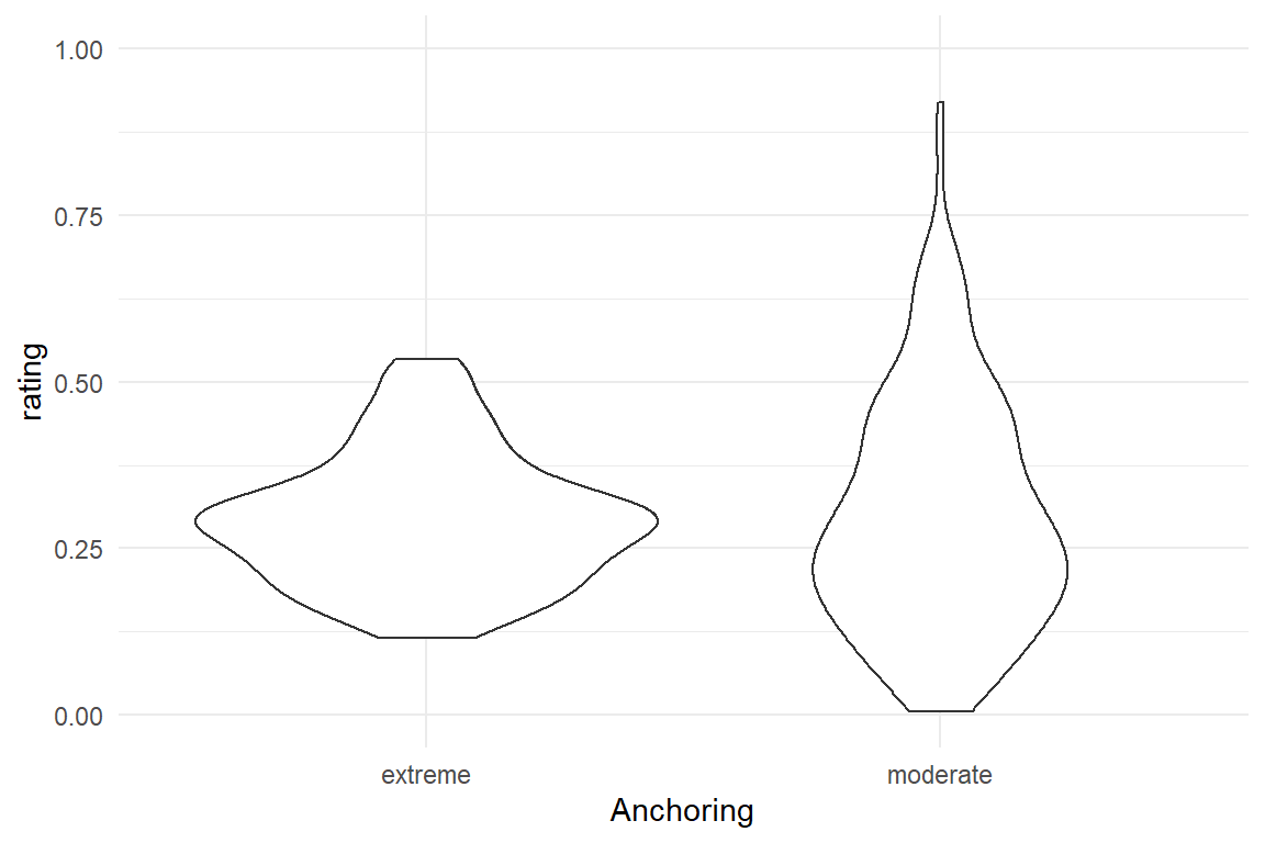
Figure 7.30: Extreme and moderate anchoring produce differently varied response distributions
Note that the rbeta command uses a different parametrization of beta distribution, with parameters a and b, which have are linked to the distribution mean and variance in rather convoluted ways.
The two response distributions have the same location, but the more narrow anchoring produces a wider dispersion of responses. How would we confirm this statistically? The Brms engine can link predictors to any other parameter of the response distribution, which the author of the package calls distributional models. They have an immense potential as they relax another assumption of GLM, namely that all variance parameters must strictly follow the mean-variance relationship demanded by a distribution family. As we have seen, one can easily create a case where this assumption is violated.
For Beta distributions, a large \(\phi\) indicates less dispersion. Accordingly, when used in a distributional model, a positive effect decreases variance.
When estimating dispersion or scale parameters, we have to regard that these are positive, strictly. The Brms engine simply extends the principle of link functions to parameters other than the \(\mu\) and sets a default log link for \(\phi\). In order to estimate the changes in \(\mu\) and \(\phi\) simultaneously, the brms engine receives two regression formulas. Having multiple formulas for a regresson model is a notable extension of the R model specification language, which is why Brms brings its own command bf() to collect these. We run a distributional Beta regression on the simulated rating scale responses:
M_beta <- brm(bf(
  rating ~ 0 + Anchoring,
  phi ~ 0 + Anchoring
),
family = Beta(),
data = D_Anchor
)
The parameter table below contains the two regular coefficients on location and, as expected, there is little difference. The intercept on scale parameter \(\phi\) is the scale in the narrow condition (with wider variance). The treatment effect on \(\phi\) is positive on the log scale, which means it deflates variance, just as expected (Table 7.26).
posterior(M_beta) %>%
  mutate(value = if_else(str_detect(parameter, "phi"),
    exp(value),
    inv_logit(value)
  )) %>%
clu()| parameter | fixef | center | lower | upper |
|---|---|---|---|---|
| b_Anchoringextreme | Anchoringextreme | 0.294 | 0.281 | 0.307 |
| b_Anchoringmoderate | Anchoringmoderate | 0.301 | 0.276 | 0.325 |
| b_phi_Anchoringextreme | 20.833 | 17.199 | 25.171 | |
| b_phi_Anchoringmoderate | 5.717 | 4.701 | 6.842 |
With such a distributional model we can discover differences in anchoring. And, even better, we can account for it. It intuitively makes sense to mix items with extreme and modest anchoring. By merging a distributional model with a designometric multi-level model 6.8.4, we can evaluate and use such heterogeneous scales. The general concept is shown in the next section, where we account for participant-level employment of scale.
7.5.2 Participant-level employment of scale
In the previous section, we have seen how to discover differences in anchoring of items. What is seen frequently in designometric studies is different response patterns in participants, in particular how much they tend to use the extremes. We can account for that by letting the variance parameter vary across participants. The following model comprises:
- a structural part for the mean with a fixed-effects polynomial term and a participant-level random effect for the response curve.
- a structural part for scale parameter
phiwith a participant-level random effect on the scale parameterphi - a Beta shape of randomness
attach(Uncanny)RK_1 <-
RK_1 %>%
mutate(response_unit = mascutils::rescale_centered(response, scale = .99) + 1)
M_poly_3_beta <-
brm(
formula = response_unit ~ 1 + huMech1 + huMech2 + huMech3 +
(1 + huMech1 + huMech2 + huMech3 | Part),
family = Beta(),
data = RK_1,
inits = 0
)
M_poly_3_beta_dist <-
brm(
formula = bf(
response_unit ~ 1 + huMech1 + huMech2 + huMech3 +
(1 + huMech1 + huMech2 + huMech3 | Part),
phi ~ 1 + (1 | Part)
),
family = Beta(),
data = RK_1,
inits = 0
)Note that on such more exotic and complex models, the regression engine sometimes has difficulties in finding valid starting values for the MCMC walk. Like here, it often helps to fix all starting values to Zero. If participants show different employment of scale, we should see that on the participant-level standard deviation of phi.
ranef(M_poly_3_beta_dist) %>%
  filter(nonlin == "phi") %>%
  mutate(Part_ord = dense_rank(center)) %>%
  ggplot(aes(x = Part_ord, y = center, ymin = lower, ymax = upper)) +
  geom_crossbar()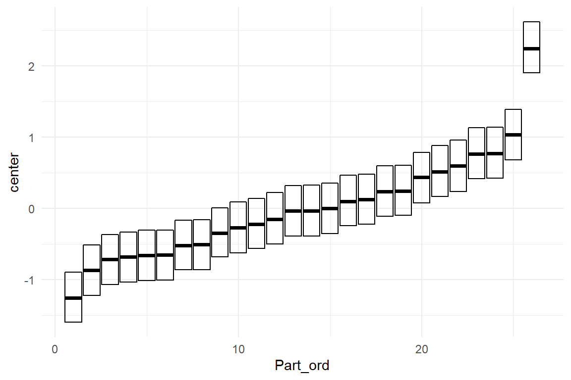
Figure 7.31: Participant-level random effects for scale parameter phi
As Figure 7.31 shows (on the linearized scale), that participants vary considerably around the population-level value of phi (\(\approx 1.4\)). While a regular Beta model adjusts the variance according to the usual mean-variance relationship, the distributional model also accounts for overall broader and narrower distributions. We would probably see some subtle adjustments in predictive plots, but this model is too complex for visual analysis (as every participant get their own phi). Therefore, we defer a deeper inspection to @ref(choos_resp), where we demonstrate the superiority of the distributional model using information criteria.
7.5.3 Participant-level skew in reaction times
In 7.3.2, the Exgaussian model seemed to sit well with reaction times, accommodating their left skew better than Gaussian or Gamma distributions. But if we review the participant-level plots carefully, we see that the shape of randomness differ between participants. There is visible differences in variance, as well as in skew.
The following distributional model estimates the same location effects (PrimeGeek), but granting all participants their own variance and skew. The maximum distributional model would estimate fully separate distributions per every participant and condition. But, since the two response distributions (Geek/nogeek) appear similar in the plots, a reduced predictor term is used, assuming that variance and shape are not affected by the experimental condition, but only the person doing the task. That is further justified by the fact, that the effect of priming categories were meager, at best.
attach(Hugme)M_1_exg_dist <-
brm(
formula = bf(
RT ~ 1 + PrimeGeek + (1 + PrimeGeek | Part),
sigma ~ 1 + (1 | Part),
beta ~ 1 + (1 | Part)
),
family = exgaussian(),
data = D_hugme,
inits = 0
)First, we extract the fixed effects, as well as the group-level standard deviation from the posterior. If participants show different patterns of randomness, we should see that in participant-level variation of \(\sigma\) and \(\beta\).
P_1_exg_dist <- posterior(M_1_exg_dist)

ranef(P_1_exg_dist) %>%
  filter(nonlin %in% c("sigma", "beta")) %>%
  group_by(nonlin) %>%
  mutate(Part_ord = dense_rank(center)) %>%
  ungroup() %>%
  ggplot(aes(x = Part_ord, y = center, ymin = lower, ymax = upper)) +
  facet_grid(~nonlin) +
  geom_crossbar()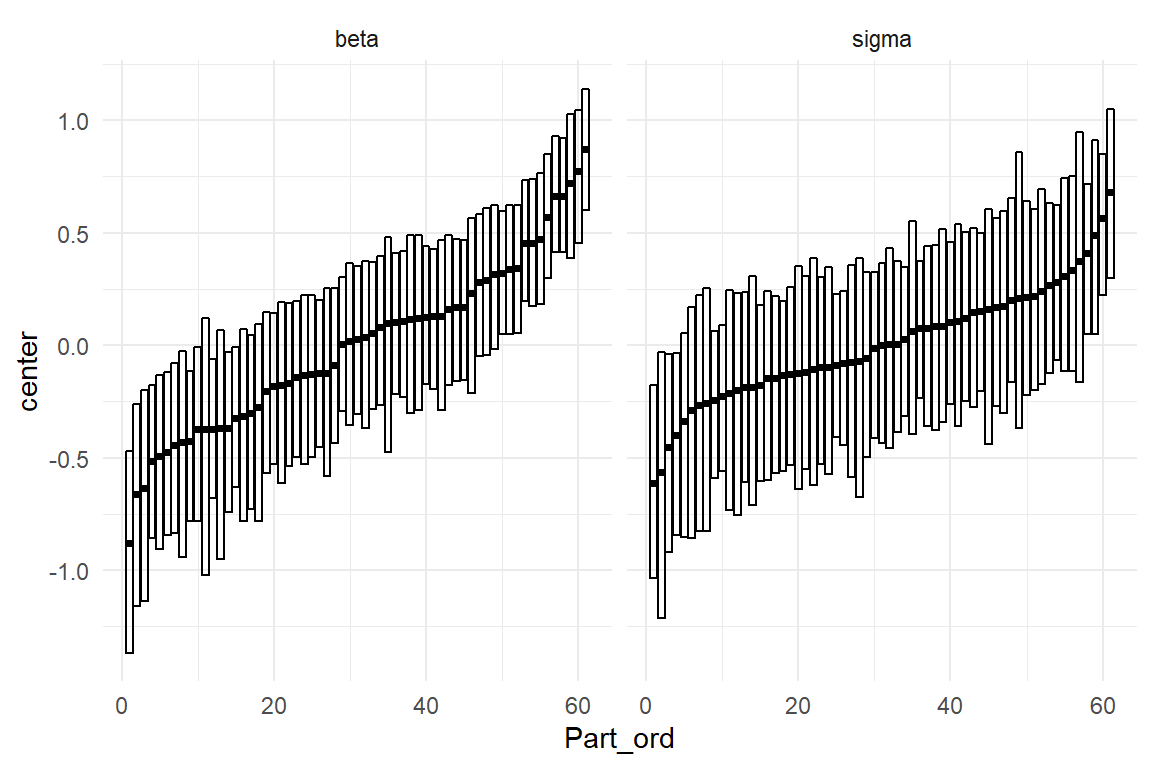
Figure 7.32: Participant-level random effects for sigma in beta
Figure 7.32 confirms, that participants vary significantly in how there RTs are dispersed (sigma), as well as how skewed they are (beta). Finally, we can also examine whether there are any associations between location, variance and skew. Recall that parameter beta gives the model the flexibility to add extra skew for when the location is far from the left boundary. If that were the case, we would see a correlation between participant-level random effects between location and skew.
P_1_exg_dist %>%
  filter(type == "ranef" & fixef == "Intercept") %>%
  mutate(
    dist_par = str_match(parameter, "beta|sigma"),
    dist_par = if_else(is.na(dist_par), "mu", dist_par)
  ) %>%
  group_by(dist_par, re_entity) %>%
  summarize(center = median(value)) %>%
  ungroup() %>%
  spread(key = dist_par, value = center) %>%
  select(-re_entity) %>%
corrr::correlate() | term | beta | mu | sigma |
|---|---|---|---|
| beta | 0.800 | 0.272 | |
| mu | 0.800 | 0.463 | |
| sigma | 0.272 | 0.463 |
One could get excited about the strong correlation between mu and beta in Table 7.27, but recall that the amount of skew introduced by beta is proportional to the location. At the same time we see a mild correlation between mu and sigma, which is just the usual mean-variance relationship, which most other distribution fanilies have already factored in. In chapter 8, we will learn how to compare models by predictive accuracy. As it will turn out in 8.2.5, the distributional Beta model in the Hugme case has a better predictive accuracy than the location-only model.
Distributional models can do more than just better accommodate data. Applied researchers and experimentalists traditionally embrace on-average effects, but have been mostly blind to effects on variance. In safety relevant systems, strong variance can be a real problem, because this implies that extremely poor performance is becoming more likely, increasing the risk of hazard. For such systems, variance is a crucial parameter and the dispersion effects of design changes should be tracked, carefully. For the readers interested in exercising this technique, several data sets from this book are candidates for such an analysis:
- CUE8: Do teams differ in the variance of ToT variance?
- Egan: What is the most robust web design (the one that reduces variance)?
- IPump: Does training (or the Novel design) reduce variance?
Experimentalists should scratch their heads, too, and take a fresh look at their theories. Systematic variation in variance can give further clues about what is going on in the minds of their participants.
In the last three chapters we have met the family of models called Generalized Multi-level Linear Models (GLMM). Linear linear models mainly rest on the linear term, a simple mechanism that unfolds into a combinatoric explosion of possibilities for the predictor side. Groudning on the idea of factors, this is conceptually further expanded by random effects and multi-level models. Multi-level models redeem variance as a first-class citizen among model parameters, and we got used to think in terms of distributions.
Generalized Linear Models expand on that perspective and deal exclusively with the response side of a model. We saw that for all design research measures the Gaussian model is wrong and an (almost) right distribution can just be identified by just following a few rules. Is it just me, or does this feel like the sudden relief, when you untie a pair of bad fitting shoes after a full day hike. And almost literally, some real pain goes away, like ordered factors for a learning curve and saturation effects.
In the recent past have seen many researchers beginning to see the beauty of the New Statistics approach. Suddenly, people start thinking of models, rather than arcane procedures, and start tinkering. Then their favorite regression engine gets a new feature, say distributional models, and it is always worth a try to improve a model.
Ironically, the abundance of possibilities leaves open the question of when to stop. How do we decide whether introducing, say distributional random effects, really improves the model? As we will see in the final chapter, there are two opposite forces at work, model complexity, which is to be avoided, and model fit. Let’s tie our shoes one more time and get a good hold!
7.6 Further readings
- In (Bürkner and Vuorre 2019) more variations of ordinal models are demonstrated using the Brms regression engine
- The extended formula interface of package Brms is explained in (Bürkner 2018), including distributional and even non-linear models.
- The Rasch model is famous in psychometrics. It can be estimated as a logistic regression model with crossed random effects for persons and items (Doran et al. 2007).