2 Getting started with R
In this book, we will be using the statistical computing environment R.
R at its core is a programming language that specializes on statistics
and data analysis. Like all modern programming languages, R comes with
a compiler or interpreter that translates human-writable formal
statements into something a computer understands and can execute. But there is much more:
R comes with a complete set of standard packages that cover common routines in statistical analysis, for
example functions to compute mean and variance, table-like data structures and the t-test. Also
regression analysis and plotting is included in R. Finally, packaged
with R comes a rudimentary programming environment, including a console,
a simple editor and a help system.
Most of what comes packaged with R, we will set aside. R is basically a brilliantly designed programming language for the task, but many of the standard packages are an inconsistent and outdated mess. For example, R comes with a set of commands to import data from various formats (SPSS, CSV, etc.). Some of these commands produce objects called data.frames, whereas others return lists of lists. Although one can convert lists into data frames, it is easier and prevents confusion if all import functions simply create data frames. As another example, to sort a data frame by participant number, one has to write the following syntax soup:
D[order(D$Part),]
In the past few years, a single person, Hadley Wickham, has started an initiative known as the tidyverse. Tidyverse first of all is a set of ground rules for dealing with data. For example, one ground rule is that all data processing routines take a data frame as input and give their results as a data frame. That may sound trivial, but it is not. Many legacy routines in R take matrices as input (or output). Matrices and data frames are both rectangular, but you can while you can convert all matrices to data frames, the opposite is not true.
The result of the dogma is a fast growing collection of libraries that all ground on a coherent and powerful set of principles for data management, and are therefor highly inter-operable. One of the core tidyverse packages is dplyr and it introduces a rich, yet rather generic, set of commands for data manipulation. The sorting of a data frame mentioned above would be written as
D %>% arrange(Part)
One of Wickham’s first and well-known contributions is the ggplot system for graphics. Think of R’s legacy graphics system as a zoo of individual routines, one for boxplots, another one for scatterplots asf. Like animals in a zoo, they live in different habitats with practically no interaction. Ggplot implements a rather abstract framework for data plots, where all pieces can be combined in a myriad of ways, using a simple and consistent syntax.
Where to get these gems? R is an open source system and has spawned an open ecosystem for statistical computing. Thousands of extensions for R have been made available by data scientists for data scientists. The majority of these packages is available through the comprehensive R archive network (CRAN). For the common user it suffices to think of CRAN as repository of packages, that can be searched and where desired packages can be downloaded and installed in an instance.
Finally, R comes with a very rudimentary programming environment that carries the questionable charm of early 1990s. Whereas several alternatives exist, most R users will feel most comfortable with the R programming environment Rstudio. At the time of writing, it is the most user-friendly and feature rich software to program in R. The next sections describe how you can set up a fully functional environment and verify that it works. Subsequently, we will get to know the basics of programming in R.
2.1 Setting up the R environment
First, we have to make sure that you have the two essential applications R and Rstudio downloaded and installed on your computer. The two programs can be retrieved from the addresses below. Make sure to select the version fit for your operating system.
If you fully own the computer you are working with, meaning that you
have administrator rights, just do the usual downloading and running of
the setup. If everything is fine, you’ll find R and Rstudio installed
under c\Programs\ and both are in your computers start menu. You can
directly proceed to the installation of packages.
In corporate environments, two issues can arise with the installation:
first a user may not have administrator rights to install programs to
the common path c:\programs\. Second, the home directory may reside on
a network drive, which is likely to cause trouble when installing
packages.
If you have no administrator rights, you must choose your home directory
during the setup. If that is a local directory, (c:/Users/YourName/),
this should work fine and you can proceed with the installation of
packages.
If your home directory (i.e. My Documents) is located on a network
drive, this is likely to cause trouble. In such a case, you must install
R and Rstudio to a local directory (on your computers hard drive), where
you have full read/write access. In the following, it is assumed that
this directory is D:/Users/YourName/:
- create a directory
D:/Users/YourName/R/. This is where both programs, as well as packages will reside. - create a sub directory
Rlibrarywhere all additional packages reside (R comes with a pack of standard packages, which are in a read-only system directory). - start Rstudio
- create a regular text file
File -> New File -> Text file - copy and paste code from the box below
- save the file as
.RprofileinD:/Users/YourName/R/ - open the menu and go to
Tools -> Global options -> General -> Default working directory. SelectD:/Users/YourName/R/.
## .Rprofile

options(stringsAsFactors = FALSE)

.First <- function() {
  RHOME <<- getwd()
  cat("\nLoading .Rprofile in", getwd(), "\n")
  .libPaths(c(paste0(RHOME, "Rlibrary"), .libPaths()))
}

.Last <- function() {
  cat("\nGoodbye at ", date(), "\n")
}
With the above steps you have created a customized start-up profile for R. The profile primarily sets the library path to point to a directory on the computers drive. As you are owning this directory, R can install the packages without admin rights. In the second part, you configure Rstudio’s default path, which is where R, invoked from Rstudio, searches for the .Rprofile.
After closing and reopening Rstudio, you should see a message in the console window saying:
Loading .Rprofile in D:/Users/YourName/R/
That means that R has found the .Rprofile file and loaded it at
start-up. The .Rprofile file primarily sets the path of the library,
which is the collection of packages you install yourself. Whether this
was successful can be checked by entering the console window in
Rstudio, type the command below and hit Enter.
.libPaths()If your installation went fine, you should see an output like the following. If the output lacks the first entry, your installation was not successful and you need to check all the above steps.
[1] “D:/Users/YourName/R/Rlibrary” “C:/Program Files/R/R-3.3.0/library”
2.1.1 Installing CRAN packages
While R comes with a set of standard packages, thousands of packages are available to enhance functionality for every purpose you can think of. Most packages are available from the Comprehensive R Network Archive (CRAN).
For example, the package foreign is delivered with R and provides functions to read data files in various formats, e.g. SPSS files. The package haven is a rather new package, with enhanced functionality and usability. It is not delivered with R, hence, so we have to fetch it.
Generally, packages need to be installed once on your system and to be loaded everytime you need them. Installation is fairly straight-forward once your R environment has been setup correctly and you have an internet connection.
In this book we will use a number of additional packages from CRAN. The
listed packages below are all required packages, all can be loaded using
the library(package) command. The package tidyverse is a metapackage
that installs and loads a number of modern packages. The ones being used
in this book are:
- dplyr and tidyr for data manipulation
- ggplot for graphics
- haven for reading and writing files from other statistical packages
- readr for reading and writing text-based data files (e.g., CSV)
- readxl for reading Excel files
- stringr for string matching and manipulation
## tidyverse
library(tidyverse)

## data manipulation
library(openxlsx)

## plotting
library(gridExtra)

## regression models
library(rstanarm)

## other
library(devtools) ## only needed for installing from Github
library(knitr)

## non-CRAN packages
library(mascutils)
library(bayr)
We start by checking the packages:
- create a new R file by
File --> New file --> R script - copy and paste the above code to that file and run it. By repeatedly
pressing
Ctrl-Returnyou run every line one-by-one. As a first time user with a fresh installation, you will now see error messages like:
Error in library(tidyverse) : there is no package called ‘tidyverse’
This means that the respective package is not yet present in your R
library. Before you can use the package tidyverse you have to install
it from CRAN. For doing so, use the built-in package management in
RStudio, which fetches the package from the web and is to be found in
the tab Packages. At the first time, you may have to select a
repository and refresh the package list, before you can find and install
packages. Then click Install, enter the names of the missing
package(s) and install. On the R console the following command downloads
and installs the package tidyverse.
install.packages("tidyverse")CRAN is like a giant stream of software pebbles, shaped over time in a growing tide. Typically, a package gets better with every version, be it in reliability or versatility, so you want to be up-to-date. Rstudio has a nice dialogue to update packages and there is the R command:
update.packages("tidyverse")Finally, run the complete code block at once by selecting it and
Ctrl-Enter. You will see some output to the console, which you should
check once again. Unless the output contains any error messages (like
above), you have successfully installed and loaded all packages.
Note that R has a somewhat idiosyncratic jargon: many languages, such
as Java or Python, call “libraries” what R calls “packages.” The
library in R is strictly the set of packages installed on your computer
and the library command loads a package from the library.
2.1.2 Installing packages from Github
Two packages, mascutils and bayr are written by the author of this book. They have not yet been committed to CRAN, but they are available on Github which is a general purpose versioning system for software developers and few authors. Fortunately, with the help of the devtools package it is rather easy to install these packages, too. Just enter the Rstudio console and type:
library(devtools)
install_github("schmettow/mascutils")
install_github("schmettow/bayr")
Again, you have to do that only once after installing R and you can
afterwards load the packages with the library command. Only if the
package gets an update to add functionality or remove bugs, you need to
run these commands again.
2.1.3 A first statistical program
After you have set up your R environment, you are ready to run your first R program (you will not yet understand all the code, but as you proceed with this book, all will become clear):
- Stay in the file where you have inserted and run the above code for loading the packages.
- Find the environment tab in Rstudio. It should be empty.
- Copy-and-paste the code below into your first file, right after library commands.
- Run the code lines one-by-one and observe what happens (in RStudio: Ctrl-Enter)
set.seed(42)
## Simulation of a data set with 100 participants
## in two between-subject conditions
N <- 100
levels <- c("control", "experimental")
Group <- rep(levels, N / 2)
age <- round(runif(N, 18, 35), 0)
outcome <- rnorm(N, 200, 10) + (Group == "experimental") * 50
Experiment <- tibble(Group, age, outcome) %>% as_tbl_obs()
Experiment| Obs | Group | age | outcome |
|---|---|---|---|
| 22 | experimental | 20 | 249 |
| 26 | experimental | 27 | 256 |
| 43 | control | 19 | 207 |
| 61 | control | 29 | 200 |
| 80 | experimental | 18 | 252 |
| 88 | experimental | 20 | 262 |
| 89 | control | 19 | 195 |
| 97 | control | 24 | 195 |
With seven lines of code you have simulated the data for an experiment with two conditions (Table 2.1). The following code produces two so-called density plots, which indicate how the simulated values are distributed along variable Outcome (Figure 2.1).
## Plotting the distribution of outcome
Experiment %>%
  ggplot(aes(x = outcome)) +
  geom_density(fill = 1)

## ... outcome by group
Experiment %>%
  ggplot(aes(fill = Group, x = outcome)) +
  geom_density()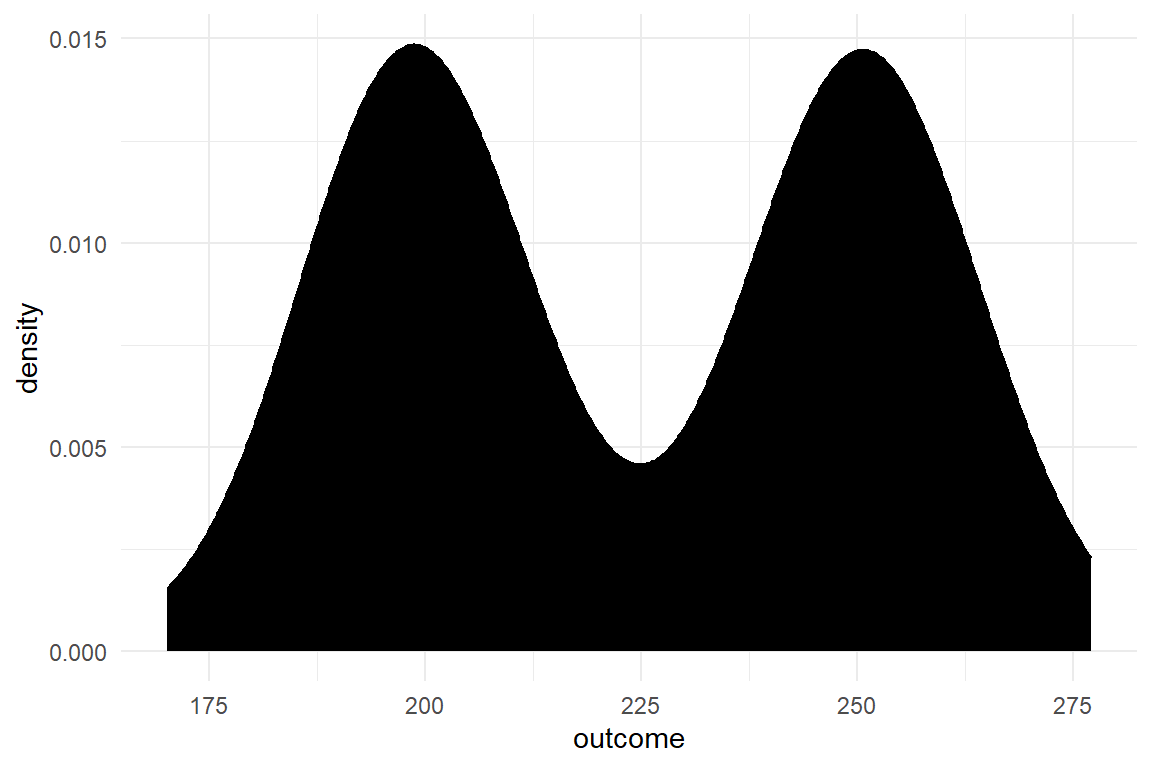
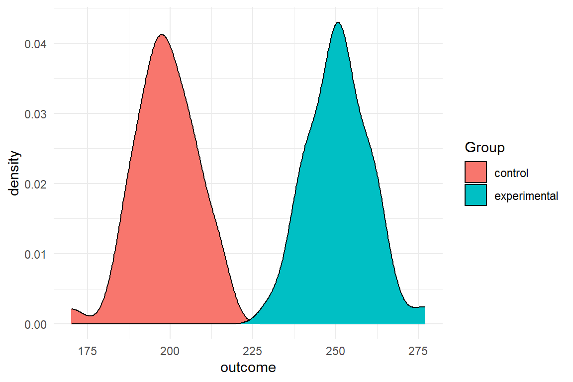
Figure 2.1: Density of simulated data
Then, we move on to estimating a statistical model and produce a summary of the estimation in Table 2.2
## ... statistical model comparing the groups

model <- stan_glm(
  formula = outcome ~ Group,
  data = Experiment
)fixef(model)| fixef | center | lower | upper |
|---|---|---|---|
| Intercept | 198.6 | 196.1 | 201.3 |
| Groupexperimental | 52.3 | 48.6 | 55.9 |
Observe Console, Environment and Plots. Did you see
- how the Environment window is populated with new variables (Values and Data)?
- a table appears in the Console, when executing the
summary(Experiment)command? - how the “camel-against-the-light” in Plots tab morphed into “two-piles-of-colored-sugar?”
Congratulations! You have just
- simulated data of a virtual experiment with two groups
- plotted the data and
- estimated a Bayesian regression model that compares the two groups.
Isn’t it amazing, that in less than 20 simple statements we have just reached the level of a second-year bachelor student? Still, you may find the R output a little inconvenient, as you may want to save the output of your data analysis. Not long ago, that really was an issue, but in the past few years R has become a great tool for reproducable research. The most simple procedure of saving your analysis for print or sharing is to:
- save the R file your have created by hitting
CTRL-Sand selecting a directory and name. - in RStudio open
File --> Compile notebookand select Word as a format. - Hit
Compile
A new Word document should appear that shows all code and the output. Now, you can copy-and-paste the graphics into another document or a presentation.
2.1.4 Bibliographic notes
Getting started with Rstudio (presentation)
Getting started with Rstudio (ebook)
rstudio cheat sheets is a collection of beautifully crafted cheat sheets for ggplot, dplyr and more. I suggest you print the data mangling and ggplot cheat sheets and always keep them on your desk.
The tidyverse is a meta package that loads all core tidyverse packages by Hadley Wickham.
2.2 Learning R: a primer
This book is for applied researchers in design sciences, whose frequent task is to analyze data and report it to stakeholders. Consequently, the way I use R in this book capitalizes on interactive data analysis and reporting. As it turns out, a small fraction of R, mostly from the tidyverse, is sufficient to write R code that is effective and fully transparent. In most cases, a short chain of simple data transformations tidies the raw data which can then be pushed into a modelling or graphics engine that will do the hard work. We will not bother (ourselves and others) with usual programming concepts such as conditionals, loops or the somewhat eccentric approaches to functional programming. At the same time, we can almost ignore all the clever and advanced routines that underlay statistical inference and production of graphics, as others have done the hard work for us.
R mainly serves three purposes, from easy to advanced: 1. interactive data analysis 2. creating data analysis reports 3. developing new statistical routines.
It turns out that creating multimedia reports in R has become very easy by the knitr/markdown framework that is neatly integrated into the Rstudio environment. I
With R one typically works interactively through a data analysis. The analysis often is a rather routine series of steps, like:
- load the data
- make a scatter plot
- run a regression
- create a coefficient table
A program in R is usually developed iteratively: once you’ve loaded and checked your data, you progress to the next step step of your analysis, test it and proceed. At every step, one or more new objects are created in the environment, capturing intermediate and final results of the analysis:
- a data frame holding the data
- a graphics object holding a scatterplot
- a model object holding the results of a regression analysis
- a data frame for the coefficient table
As R is an interpreter language, meaning there is no tedious compile-and-run cycles in everyday R programming. You develop the analysis as it happens. It is even normal to jump back and forth in an R program, while building it.
R is a way to report and archive what precisely you have been doing with your data. In statistics, mathematical formulas are the common form of unambiguously describing a statistical model. For example, the following equation defines a linear regression model between the observed outcome \(y\) and the predictor \(x\):
\[ \begin{aligned} \mu_i &= \beta_0 + \beta_1x_i\\ y_i &\sim N(\mu_i, \sigma) \end{aligned} \]
As we will later see 4.3.1, in Rs formula language the same model is unambiguously specified as:
y ~ x
R is currently the lingua franca of statistical computing. As a programming language, R has the same precision as math, but is more expressive. You can specify complex models, but also graphics and the steps of data checking and preparation. As an example, consider an outlier removal rule of:
An observation is valid if it does not exceed the tenfold of the observation mean.
We just applied our own rule of outlier removal to the data. Others may consider this rule invalid or arbitrary. Disagreement is virtue in science and one can only disagree with what one actually sees. In R, the researcher formally reports what precisely has been done with the data. For example, the same outlier removal rule is unambiguously specified by the following code (the first line just simulates some data). The results are shown in Table 2.3.
D <- tibble(score = c(1, 2, 4, 3, 5, 6, 50, 800)) %>%
  as_tbl_obs()

D %>% filter(score < mean(score))| Obs | score |
|---|---|
| 1 | 1 |
| 2 | 2 |
| 3 | 4 |
| 4 | 3 |
| 5 | 5 |
| 6 | 6 |
| 7 | 50 |
Finally, R is a way to develop and share statistical programs. Thousands of packages in the R ecosystem cover almost all statistical problems you can imagine. As a programming language, R has been designed for that particular purpose. Under the hood of R, a bunch of generic, yet powerful, principles purr to make it a convenient language for typical problems in statistical computation. Readers with programming experience can fly over the R basics that follow. But, as a specific purpose language R has a few idiosyncracies you should know about:
Almost all programming languages the first element of a list has the index zero. We got used to it, but for beginners it is a another hurdle that is unnecessary. Mathematicians, catholiques, software developers in bars and everyone, young or old, counts
“one,” “two” ,“three.”
And so does R:
c(1:3)[1:3]## [1] 1 2 3Counting from one is perhaps the most lovable idiosyncracy of R. But, lets also welcome people who have experience with other programming languages:
The first thing one has to know about R is that it is a functional programming language. A function simply is a programmed procedure that takes data as input, applies some transformation and returns data as output. That sounds trivial, but there is an important difference to most other languages: Different to procedures in Pascal or object oriented methods (in Java or Python), functions are forbidden to modify any external object. A certain function is a black box, but one can be sure that the only thing it does is return a new object.
At the same time, functions are first-class citizens in R and can be
called everywhere, even as an argument to another function. The purrr
package is famous for functions that call functions, also called
high-level functions, such as map, or rerun.
The routine application of higher level functions is to apply a transformation to a list of objects. In a majority of programming languages you would put this in a loop and this is where programmers often have to re-learn, when they get started with R. Believe me one thing: Once you have wrapped your head around functional programming, you will program the same procedure in a quarter of time with half the code and your program will run significantly faster. My general advice is:
Whenever you think you need a loop, you don’t.
For me it helped to imagine the following: loops carry the notion of chain of data that moves over a fixed transformation device. In functional programing functions the can work in a hierarchy, a high-level device moves along a string of data. It carries an exchangeable low-level device that applies the desired transformation to every position.
If you come from relational data bases you you have something in common with the statistician: you both think in transformation of tables. Not coincidently, the features in dplyr, the tidy data transformation engine, are clearly borrowed from SQL. You will also feel at home with the idea of reports powered by functional chunks embedded in a templating system.
For object orientation folks, R is a good choice, but you have to get used to it. First, it gives you the choice of several object orientation systems, which sometimes requires to install a package. The so-called S3 system is the original. It is rather limited and some even call it informal. The approach is as simple as it is unusal. At its heart it is a methods dispatcher that handles inheritance and overloading of functions. S3 puts methods first, whereas objects of a class simply get a tag for the dispatcher.
Beginners are at peace with all of this. You can count like you do.
Functional programming is intuitive for working on data. And
because of S3 the function summary always does something useful.
2.2.1 Assigning and calling Objects
Any statistical analysis can be thought of as a production chain. You take the raw data and process it into a neat data table, which you feed into graphics and regression engines or summarize by other means. At almost every step there is an input and an output object.
Objects are a basic feature of R. They are temporary storage places in
the computer’s memory. Objects always have a name chosen by the
programmer. By its name, a stored object can be found back at any time.
Two basic operations apply for all objects: an object is stored by
assigning it a name and it is retrieved by calling its name. If you
wanted to store the number of observations in your data set under the
name N_obs, you use the assignment operator <-. The name of the
variable is left of the operator, the assigned value is right of it.
N_obs <- 100Now, that the value is stored, you can call it any time by simply calling its name:
N_obs## [1] 100Just calling the name prints the value to Console. In typical interactive programming sessions with R, this is already quite useful. But, you can do much more with this mechanism.
Often, what you want is to do calculations with the value. For example,
you have a repeated measures study and want to calculate the average
number of observations per participant. For this you need the number of
observations, and the number of participants. The below code creates
both objects, does the calculation (right of <-) and stores it in
another object avg_N_Obs
N_Obs <- 100
N_Part <- 25
avg_N_Obs <- N_Obs / N_Part
avg_N_Obs
## [1] 4Objects can exist without a name, but are volatile, then. They cannot be used any further. The following arithmetic operation does create an object, a single number. For a moment or so this number exists somewhere in your computers memory, but once it is printed to the screen, it is gone. Of course, the same expression can be called again, resulting in the same number. But, strictly, it is a different object.
N_Obs / N_Part ## gone after printing## [1] 4N_Obs / N_Part ## same value, different object## [1] 4There even is a formal way to show that the two numbers, although having the same value assigned, are located at different addresses. This is just for the purpose of demonstration and you will rarely use it in everyday programming tasks:
tracemem(N_Obs / N_Part)## [1] "<00000000A50E40F0>"tracemem(N_Obs / N_Part)## [1] "<00000000A5114C40>"2.2.2 Vectors
Notice the [1] that R put in front of the single value when printing
it? This is an index. Different to other programming languages, all
basic data types are vectors in R. Vectors are containers for storing
many values of the same type. The values are addressed by the index,
N_Obs[1] calls the first element. In R, indices start counting with
1, which is different to most other languages that start at zero. And
if you have a single value only, this is just a vector of length one.
For statistics programming having vectors as basic data types makes perfect sense. Any statistical data is a collection of values. What holds for data is also true for functions applied to data. Practically all frequently used mathematical functions work on vectors, take the following example:
X <- rnorm(100, 2, 1)
mean(X)
## [1] 1.99The rnorm command produces a vector of length 100 from three values.
More precisely, it does 100 random draws from a normal distribution with
mean 2 and an SD of 1. The mean command takes the collection and
reduces it to a single value. By the way, this is precisely, what we
call a statistic: a single quantity that characterizes a collection of
quantities.
2.2.3 Basic object types
Objects can be of various classes. In R the common basic classes are: logical, factor, character, integer and numeric. Besides that, programmers can define their own complex classes, for example, to store the results of regression models.
Objects of type logical store the two levels TRUE, FALSE, like
presence or absence of a treatment, or passed and failed test items.
With Boolean operators one can compute new logical values, for example:
Apple <- TRUE
Pear <- FALSE

Apple & Pear ## and
## [1] FALSEApple | Pear ## or## [1] TRUEMore generally, logical values can be used for categorization, when
their are only two categories, which is called a dichotomous variable.
For example, gender is usually coded as a vector of characters
("m", "f", "f"), but one can always do:
is_female <- c(FALSE, TRUE, TRUE)
is_male <- c(T, F, F)
Programmers are lazy folks when it comes to typing, therefore R allows
you to abbreviate TRUE and FALSE as shown above. As a consequence,
one should never assign objects the name reserved for logical values, so
don’t do one of the following:
## never do this
TRUE <- "All philosophers have beards"
F <- "All gods existed before the big bang"
42 * F
The class numeric stores real numbers and is therefore abundant in
statistical programming. All the usual arithmetic operations apply:
a <- 1.0
b <- a + 1
sqrt(b)
## [1] 1.41Objects of class integer are more specific as they store natural
numbers, only. This often occurs as counts, ranks or indices.
friends <- c(
  anton = 1,
  berta = 3,
  carlo = 2
)
order(friends)
## [1] 1 3 2The usual arithmetic operations apply, although the result of operation
may no longer be integer, but numeric
N <- 3
sum_of_scores <- 32
mean_score <- 32 / 3
mean_score
## [1] 10.7class(mean_score)## [1] "numeric"Surprisingly, logical values can be used in arithmetic expressions, too.
When R encounters value TRUE in an arithmetic context, it replaces it
with 1, zero otherwise. Used with multiplication, this acts like an
on/off switch, which we will put to use for building factorial
models.
TRUE + TRUE## [1] 2sqrt(3 + TRUE)## [1] 2is_car <- c(TRUE, TRUE, FALSE) ## bicycle otherwise
wheels <- 2 + is_car * 2
wheels## [1] 4 4 2Data sets usually contain variables that are not numeric, but partition the data into groups. For example, we frequently group observations by the following
Part: participantCondition: experimental conditionDesign: one of several designsEducation: level of education (e.g., low, middle or high)
Two object types apply for grouping observations: factor and character. While factors specialize on grouping observations, character objects can also be used to store longer text, say the description of a usability problem. The following identifies two conditions in a study, say a comparison of designs A and B. Note how the factor identifies its levels when called to the screen:
design_char <- c("A", "B", "B", "A")
design_char
## [1] "A" "B" "B" "A"design_fact <- factor(c("A", "B", "B", "A"))
design_fact## [1] A B B A
## Levels: A BStatistical analyses deal with real world data which ever so often is
messy. Frequently, a planned observation could not be recorded, because
the participant decided to quit or the equipment did not work properly
or the internet collapsed. Users of certain legacy statistics packages
got used to coding missing observations as -999 and then declared this
a missing value. In R missing values are first-class citizens. Every
vector of a certain class can contain missing values, which are
identified as NA.
Most basic statistics functions, like mean(), sd() or median() are
act conservatively when the data contains missing values. If there is a
single NA in the variable to be summarized, the result is NA. While
this is good in the sense of transparency, much of the time what the
researcher wants is to have the summary statistic with NA values being
removed, first.
clicks <- c(3, NA, 2)
mean(clicks)
## [1] NAmean(clicks, na.rm = T)## [1] 2.5This book is about programming and statistics at the same time. Unfortunately, there are a few terms that have a particular meaning in both domains. One of those is a “variable.” In statistics, a variable usually is a property we have recorded, say the body length of persons, or their gender. In general programming, a variable is a space in the computers memories, where results can be stored and recalled. Fortunately, R avoids any confusion and calls objects what is usually called a programming variable.
2.2.4 Operators and functions
R comes with a full bunch of functions for creating and summarizing
data. Let me first introduce you to functions that produce exactly one
number to characterize a vector. The following functions do that with to
the vector X, every in their own way:
length(X)
sum(X)
mean(X)
var(X)
sd(X)
min(X)
max(X)
median(X)
These functions are a transformation of data. The input to these
transformations is X and is given as an argument to the function.
Other functions require more than one argument. The quantile function
is routinely used to summarize a variable. Recall that X has been
drawn from a Normal distribution of \(\mu=2\) and standard deviation
\(\sigma = 1\). All Normal distributions have the property that about 66%
of the mass is within the range of \(\mu-\sigma\) and \(\mu+\sigma\)
. That means in turn: 17% are below \(\mu-\sigma\) and 66 + 17
= 83% are below \(\mu+\sigma\). The number of observations in a certain
range of values is called a quantile. The quantile function operates
on X, but takes an (optional) vector of quantiles as second argument:
quantile(X, c(.17, .83))## 17% 83%
## 0.963 2.956Most functions in R have optional arguments that let you change how
the function performs. The basic mathematical functions all have the
optional argument na.rm. This is a switch that determines how the
function deals with missing values NA. Many optional arguments have
defaults. The default of na.rm is FALSE (“return NA in case of NAs
in the vector”). By setting it to TRUE, they are removed before
operation.
B <- c(1, 2, NA, 3)
mean(B)
## [1] NAmean(B, na.rm = TRUE)## [1] 2Most more complex routines in R have an abundance of parameters, most of
which have reasonable defaults, fortunately. To give a more complex
example, the first call of stan_glm performs a Bayesian estimation of
the grand mean model. The second does a Poisson grand mean model with
5000 iterations per MCMC chain. As seed has been fixed, every
subsequent run will produce the exact same chains. My apologies for the
jargon!
D_1 <- tibble(X = rnorm(20, 2, 1))
M_1 <- stan_glm(X ~ 1,
  data = D_1
)

D_2 <- tibble(X = rpois(20, 2))
M_2 <- stan_glm(X ~ 1,
  family = poisson,
  seed = 42,
  iter = 5000,
  data = D_1
)
R brings the usual set of arithmetic operators, like +, -, *, /
and more. In fact, an operator is just a function. The sum of two
numbers can, indeed, be written in these two ways:
1 + 2## [1] 3`+`(1, 2)## [1] 3The second term is a function that takes two numbers as input and returns a third. It is just a different syntax, and this one is called the polish notation. I will never use it throughout the rest of this book.
Another set of commonly used operators are logical, they implement Boolean algebra. Some common Boolean operators are shown in the truth table (Table 2.4).
| A | B | !A | A & B | A | B | A == B |
|---|---|---|---|---|---|
| not | and | or | equals | ||
| T | T | F | T | T | T |
| T | F | F | F | T | F |
| F | T | T | F | T | F |
| F | F | T | F | F | T |
Be careful not to confuse Boolean “and” and “or” with their common natural language use. If you ask: “Can you buy apples or pears on the market?” the natural answer would be: “both.” The Boolean answer is: TRUE. In a requirements document you could state “This app is for children and adults.” In Boolean the answer would be FALSE, because no one can be a child and an adult at the same time, strictly. A correct Boolean statement would be: “The envisioned users can be adult or child.”
Further Boolean operators exist, but can be derived from the three
above. For example, the exclusive OR, “either A or B” can be written as:
(A | B) & !(A & B). This term only gets TRUE when A or B is TRUE, but
not both. In the data analysis workflow, Boolean logic is frequently
used for filtering data and we re-encounter them in data transformation.
Finally, it sometimes is convenient or necessary to program own functions. A full coverage of developing functions is beyond the scope of this introduction, so I show just one simple example. If one desires a more convenient function to compute the mean that ignore missing values by default, this can be constructed as follows:
mean_conv <- function(x) {
  mean(x = B, na.rm = TRUE)
}

mean_conv(B)
## [1] 2Notice that:
- the
function()function creates new functions - the arguments given to
function(x)will be the arguments expected by the functionmean_conv(x). - code enclosed by
More examples of creating basic functions can be found in section 3.3. As R is a functional programming language, it offers very elaborate ways of programming functions, way beyond what is found in common languages, such as Python or Java. An advanced example is given in section 8.2.2.
2.2.5 Storing data in data frames
Most behavioral research collects real data to work with. As behavior researchers are obsessed about finding associations between variables, real data usually contains several. If you have a sample of observations (e.g. participants) and every case has the same variables (measures or groups), data is stored in a table structure, where columns are variables and rows are observations.
R knows the data.frame objects to store variable-by-observation
tables. Data frames are tables, where columns represent statistical
variables. Variables have names and can be of different data types, as
they usually appear in empirical research. In many cases data frames are
imported to R, as they represent real data. Here, we first see how to
create data frames by simulation. First, we usually want some initial
inspection of a freshly harvested data frame.
Several commands are available to look into a data frame from different
perspectives. Another command that is implemented for a variety of
classes, ibluding dara frames, is summary. For all data frames, it
produces an overview with descriptive statistics for all variables (i.e.
columns), matching their object type. Particularly useful for data
initial screening, is that missing values are listed per variable.
print(summary(Experiment))## Obs Group
## Min. : 1.0 Length:100
## 1st Qu.: 25.8 Class :character
## Median : 50.5 Mode :character
## Mean : 50.5
## 3rd Qu.: 75.2
## Max. :100.0
## age outcome
## Min. :18.0 Min. :170
## 1st Qu.:22.0 1st Qu.:199
## Median :27.5 Median :223
## Mean :27.0 Mean :225
## 3rd Qu.:31.0 3rd Qu.:251
## Max. :35.0 Max. :277The str (structure) command works on any R object and displays the
hierarchical structure (if there is one):
str(Experiment)## tbl_obs [100 x 4] (S3: tbl_obs/tbl_df/tbl/data.frame)
## $ Obs : int [1:100] 1 2 3 4 5 6 7 8 9 10 ...
## $ Group : chr [1:100] "control" "experimental" "control" "experimental" ...
## $ age : num [1:100] 34 34 23 32 29 27 31 20 29 30 ...
## $ outcome: num [1:100] 203 242 216 256 201 ...Data frames store variables, but statistical procedures operate on variables. We need ways of accessing and manipulating statistical variables and we will have plenty. First, recall that in R the basic object types are all vectors. You can store as many elements as you want in an object, as long as they are of the same class.
Internally, data frames are a collection of “vertical” vectors that are
equally long. Being a collection of vectors, the variables of a data
frame can be of different classes, like character, factor or
numeric. In the most basic case, you want to calculate a statistic for
a single variable out of a data frame. The $ operator pulls the
variable out as a vector:
mean(Experiment$outcome)## [1] 225As data frames are rectangular structures, you can also access individual values by their addresses. The following commands produce three sub-tables of Experiment (Table 2.5):
- the first outcome measure
- the first three rows of Group
- the complete first row
Experiment[1, 3]
Experiment[1:3, 2]
Experiment[1, ]
|
|
|
Addressing one or more elements in square brackets, always requires two
elements, first the row, second the column. As odd as it looks, one or
both elements can be empty, which just means: get all rows (or all
columns). Even the expression Experiment[,] is fully valid and will
just the return the whole data frame.
There is an important difference, however, when using R’s classic
data.frame as compared to dplyr’s tibbleimplementation: When using
single square brackets on dplyr data frames one always gets a data frame
back. That is a very predictable behavior, and very much unlike the
classic: with data.frame, when the addressed elements expand over
multiple columns, like Experiment[, 1:2], the result will be a
data.frame object, too. However, when slicing a single column, the
result is a vector:
Exp_classic <- as.data.frame(Experiment)
class(Exp_classic[1:2, 1:2]) ## data.frame
## [1] "data.frame"class(Exp_classic[1, ]) ## data.frame## [1] "data.frame"class(Exp_classic[, 1]) ## vector## [1] "integer"Predictability and a few other useful tweaks made me prefer tibble
over data.frame. But, many third-party packages continue to produce
classic data.frame objects. For example, there is an alternative to
package `readxl, openxlsx, which reads (and writes) Excel files. It
returns classic data.frames, which can easily be converted as follows:
D_foo <-
  read.xlsx("foo.xlsx") %>%
  as_tibble()
If you slice a Tibble, the results is always a Tibble, even if you pick a single cell.
Sometimes, one wants to truly extract a vector. With a tibble a single
column can be extracted as a vector, using double square brackets, or
using the $ operator.
Experiment[[1]] ## vector
Experiment$Group ## the same
Sometimes, it may be necessary to change values in a data frame. For
example, a few outliers have been discovered during data screening, and
the researcher decides to mark them as missing values. The syntax for
indexing elements in a data frame can be used in conjunction with the
assignment operator <-. In the example below, we make the simulated
experiment more realistic by injecting a few outliers. Then we discard
these outliers by setting them all to NA.
## injecting
Experiment[2, "outcome"] <- 660
Experiment[6, "outcome"] <- 987
Experiment[c(1, 3), "age"] <- -99

## printing first few observations
head(Experiment)| Obs | Group | age | outcome |
|---|---|---|---|
| 1 | control | -99 | 203 |
| 2 | experimental | 34 | 660 |
| 3 | control | -99 | 216 |
| 4 | experimental | 32 | 256 |
| 5 | control | 29 | 201 |
| 6 | experimental | 27 | 987 |
## setting to NA (by injection)
Experiment[c(2, 6), "outcome"] <- NA
Experiment[c(1, 3), "age"] <- NA
Besides injection, note two more features of addressing data frame
elements. The first is, that vectors can be used to address multiple
rows, e.g. 2 and 6. In fact, the range operator 1:3 we used above is
just a convenient way of creating a vector c(1,2,3). Although not
shown in the example, this works for columns alike.
The careful reader may also have noted another oddity in the above
example. With Experiment[c(2, 6),"outcome"] we addressed two elements,
but right-hand side of <- is only one value. That is a basic mechanism
of R, called reuse. When the left-hand side is longer than the
right-hand side, the right-hand side is reused as many times as needed.
Many basic functions in R work like this, and it can be quite useful.
For example, you may want to create a vector of 20 random
numbers, where one half has a different mean as the second half of
observations.
rnorm(20, mean = c(1, 2), sd = 1)The above example reuses the two mean values 50 times, creating an
alternating pattern. Strictly speaking, the sd = 1 parameter is
reused, too, a 100 times. While reuse often comes in convenient, it can
also lead to difficult programming errors. So, it is a good advice to be
aware of this mechanism and always carefully check the input to
vectorized functions.
2.2.6 Import, export and archiving
R lets you import data from almost every conceivable source, given that
you have installed and loaded the appropriate packages (foreign, haven
or openxlsx for Excel files). Besides that R has its own file format for
storing data, which is .Rda files. With these files you can save data
frames (and any other object in R), using the
save(data, file = "some_file.Rda") and load(file = "some_file.Rda")
commands.
Few people create their data tables directly in R, but have legacy data sets in Excel (.xslx) and SPSS files (.sav). Moreover, the data can be produced by electronic measurement devices (e.g. electrodermal response measures) or programmed experiments can provide data in different forms, for example as .csv (comma-separated-values) files. All these files can be opened by the following commands:
## Text files
Experiment <-
  read_csv("Data/Experiment.csv") %>%
  as_tbl_obs()

## Excel
Experiment <-
  read_excel("Data/Experiment.xlsx", sheet = 1) %>%
  as_tbl_obs()

## SPSS (haven)
Experiment <-
  read_sav("Data/Experiment.sav") %>%
  as_tbl_obs()

## SPSS (foreign)
Experiment <-
  read.spss("Data/Experiment.sav", to.data.frame = TRUE) %>%
  as_tbl_obs()
Note that I gave two options for reading SPSS files. The first (with an
underscore) is from the newer haven package (part of tidyverse). With
some SPSS files, I experienced problems with this command, as it does
not convert SPSS’s data type labelled (which is almost the same as an
R factor). The alternative is the classic read.spss command which
works almost always, but as a default it creates a list of lists, which
is not what you typically want. With the extra argument, as shown, it
behaves as expected.
This is also a good moment to address the notorious as_tbl_obs(),
whenever I simulate or read data. The command is from the Bayr package.
Its main purpose is to produce a useful display of what is in the data.
A regular Tibble (or Data.frame) object puts the whole data table into your
report. I you first call it a table of observations (tbl_obs), it will
only print eight randomly selected observations (rows), plus, hold our breath,
automatic table captions in your report. The second function of as_tbl_obs()
is to add a variable Obs, which is just a sequential identifier.
Remember, data frames are objects in the memory of your computer; and as such volatile. Once you leave your R session, they are gone. Once you have a data frame imported and cleaned, you may want to store it to a file fopr future use. Like for reading, many commands are available for writing all kinds of data formats. If your workflow is completely based on R, you can conveniently use R’s own format for storing data, Rdata files (Rda). For storing a data frame and then reading it back in (in your next session), simply do:
save(Experiment, file = "Data/Experiment.Rda")
load(file = "Data/Experiment.Rda")
Note that with save and load all objects are restored by their
original names, without using any assignments. Take care, as this will
not overwrite any object with the same name. Another issue is that for
the save command you have to explicitly refer to the file argument
and provide the file path as a character object. In Rstudio, begin
typing file="", put the cursor between the quotation marks and hit
Tab, which opens a small dialogue for navigation to the desired
directory.
Once you have loaded, prepared and started to analyze a data frame in R,
there is little reason to go back to any legacy program. Still, the
haven and foreign packages contain commands to write to various file
formats. I’ll keep that as an exercise to the reader.
2.2.7 Case environments
This book features more than a dozen case studies. Every case will be
encountered several times and multiple objects are created along the
way: data sets, regressions, graphics, tables, you name it. That posed
the problem of naming the objects, so that they are unique. I could have
chosen object names, like: BrowsingAB_M_1, AUP_M_1, etc. But, this
is not what you normally would do, when working on one study at a time.
Moreover, every letter you add to a line of code makes it more prone to
errors and less likely that you, dear reader, are typing it in and
trying it out yourself.
For these reasons, all cases are enclosed in case environments and provided with this book. For getting a case environment to work in your session, it has to be loaded from the respective R data file first:
load("BrowsingAB.Rda")In R, environments are containers for collections of objects. If an
object BAB1 is placed in an environment BrowsingAB, it can be called
as BrowsingAB$BAB1. This way, no brevity is gained. Another way to
assess objects in an environment is to attach the environment first as:
attach(BrowsingAB)
BAB1| Obs | Part | Task | Design | Gender | Education | age | Far_sighted | Small_font | ToT | clicks | returns | rating | age_shft | age_cntr |
|---|---|---|---|---|---|---|---|---|---|---|---|---|---|---|
| 53 | 53 | 1 | A | M | High | 64 | FALSE | FALSE | 33.3 | 1 | 0 | 2 | 44 | 13.83 |
| 59 | 59 | 1 | A | F | Middle | 63 | FALSE | FALSE | 152.6 | 4 | 3 | 4 | 43 | 12.83 |
| 69 | 69 | 1 | A | M | Middle | 74 | TRUE | FALSE | 146.4 | 8 | 0 | 3 | 54 | 23.83 |
| 125 | 125 | 1 | B | F | Low | 50 | FALSE | TRUE | 76.0 | 2 | 0 | 2 | 30 | -0.17 |
| 166 | 166 | 1 | B | M | High | 62 | FALSE | TRUE | 44.9 | 0 | 0 | 1 | 42 | 11.83 |
| 170 | 170 | 1 | B | F | Middle | 47 | FALSE | TRUE | 18.0 | 1 | 1 | 2 | 27 | -3.17 |
| 187 | 187 | 1 | B | M | Middle | 43 | TRUE | TRUE | 161.7 | 6 | 2 | 3 | 23 | -7.17 |
| 190 | 190 | 1 | B | F | Low | 60 | FALSE | TRUE | 111.3 | 3 | 2 | 2 | 40 | 9.83 |
Calling attach gets you into the namespace of the environment
(formally correct: the namespace gets imported to your working
environment). All objects in that namespace become immediately visible
by their mere name. The detach command leaves the environment, when you are done.
When working with the case environments, I strongly recommend to detach
before attaching another environment.
All case environments provided with this book contain one or more data
sets. Many of the cases are synthetic data which has been generated by a
simulation function. This function, normally called simulate, is
provided with the case environment, too. That gives you the freedom to
produce your own data sets with the same structure, but different
effects. Generally, calling the simulation function without any further
arguments, exactly reproduces the synthetic data set provided with the
case environment.
simulate() ## exactly reproduces the data frame BAB1Simulation functions have a parameters by which you can tune the data generating process.
Table 2.8 shows a data set of only six ToT observations. These observations are
perfect in a sense, because sd = 0 effectively removed the random component.
simulate(n_Part = 6, sd_epsilon = 0) ## just 6 observations| Obs | Part | Task | Design | Gender | Education | age | Far_sighted | Small_font | ToT | clicks | returns | rating |
|---|---|---|---|---|---|---|---|---|---|---|---|---|
| 25 | 1 | 5 | A | F | Middle | 56 | TRUE | FALSE | 191.7 | 10 | 3 | 5 |
| 43 | 1 | 3 | B | F | Middle | 56 | TRUE | TRUE | 232.6 | 12 | 5 | 6 |
| 2 | 2 | 1 | A | F | Middle | 42 | TRUE | FALSE | 110.5 | 7 | 2 | 3 |
| 14 | 2 | 3 | A | F | Middle | 42 | TRUE | FALSE | 163.8 | 8 | 1 | 4 |
| 56 | 2 | 5 | B | F | Middle | 42 | TRUE | TRUE | 139.1 | 11 | 0 | 4 |
| 28 | 4 | 5 | A | F | High | 22 | TRUE | FALSE | 107.1 | 3 | 0 | 3 |
| 34 | 4 | 1 | B | F | High | 22 | TRUE | TRUE | 89.6 | 4 | 1 | 2 |
| 24 | 6 | 4 | A | M | Low | 45 | FALSE | FALSE | 103.1 | 7 | 1 | 2 |
Furthermore, once you delve deeper into R, you can critically inspect the simulation function’s code for its behavioral and psychological assumptions (working through the later chapters on data management and simulation will help).
simulate ## calling a function without parentheses prints codeFinally, the case environments contain all objects that have been created throughout this book. This is especially useful for the regression models, as fitting these can take from a few seconds to hours.
Note that working with environments is a tricky business. Creating these
case environments in an efficient way was more difficult than you may
think. Therefore, I do not recommend using environments in everday
data analysis, with one exception: at any moment the current working
environment contains all objects that have been created, so far. That is
precisely the set of objects shown in the Environment pane of Rstudio
(or call ls() for a listing). Saving all objects and retrieving them
when returning from a break is as easy as:
save(file = "my_data_analysis.Rda")
## have a break
load("my_data_analysis.Rda")
Next to that, Rstudio can be configured to save the current workspace on exit and reload it on the next start. When working on just one data analysis for a longer period of time, this can be a good choice.
2.2.8 Structuring data
In the whole book, data sets are structured according to the rule one-row-per-observation of the dependent variable (the ORPO rule). Many researchers still organize their data tables as one-row-per-participant, as is requested by some legacy statistics programs. This is fine in research with non-repeated measures, but will not function properly with multi-level data sets. Consider a study where two designs were evaluated by three participants using a self-report item, like “how easy to use is the interface?” Then, the wrong way of structuring the data would be as in Table 2.9, without multiple observations per row (A and B).
ORPO %>%
  # filter(Task == 1, Item == 1) %>%
  # mascutils::discard_redundant() %>%
  sample_n(8) %>%
spread(Design, response) | Part | Task | Item | A | B |
|---|---|---|---|---|
| 1 | 1 | 2 | 4 | |
| 2 | 1 | 2 | 2 | |
| 2 | 2 | 1 | 4 | |
| 2 | 2 | 2 | 3 | |
| 3 | 1 | 1 | 4 | |
| 3 | 1 | 3 | 1 | |
| 3 | 2 | 3 | 6 | 2 |
ORPO %>% as_tbl_obs()| Obs | Part | Task | Design | Item | response |
|---|---|---|---|---|---|
| 1 | 1 | 1 | A | 1 | 3 |
| 16 | 1 | 2 | A | 2 | 7 |
| 28 | 1 | 2 | A | 3 | 6 |
| 31 | 1 | 1 | B | 3 | 4 |
| 2 | 2 | 1 | A | 1 | 3 |
| 8 | 2 | 1 | B | 1 | 6 |
| 17 | 2 | 2 | A | 2 | 3 |
| 33 | 3 | 1 | B | 3 | 1 |
The correct way structure is shown in Table 2.10. But, the ORPO rule dictates another principle: every row should have a unique identifier (besides the observation ID), which often is a combination of values. In the example above, every observation is uniquely identified by the participant identifier and the design condition. If we extend the example slightly, it is immediately apparent, why the ORPO rule is justified. Imagine, the study actually asked three participants to rate two different tasks on two different designs by three self-report items. By the ORPO rule, we can easily extend the data frame as below (showing a random selection of rows). I leave it up to the reader to figure out how to press such a data set in the wide legacy format.
Using identifiers is good practice for several reasons. First, it reduces problems during manual data entry. Second, it allows to efficiently record data in multi-method experiments and join them automatically. Lastly, the identifiers will become statistically interesting by themselves when we turn to linear mixed-effects models and the notion of members of a population 6.5. Throughout the book I will use standard names for recurring identifier variables in design research:
- Part
- Design
- Item
- Task
Note that usually these entities get numerical identifiers, but these numbers are just labels. Throughout, variables are written Uppercase when they are entities, but not real numbers. An exception is the trial order in experiments with massive repeated measures. These get a numerical type to allow exploring effects over time such as learning, training and fatigue.
2.2.9 Data transformation
Do you wonder about the strange use of %>% in my code above? This is
the tidy way of programming data transformations in R.
The so-called magritte operator %>% is part of the dplyr/tidyr
framework for data manipulation. It chains steps of data manipulation by
connecting transformation functions, also called piping. In the
following, we will first see a few basic examples. Later, we will
proceed to longer transformation chains and see how graceful dplyr
piping is, compared to the classic data transformation syntax in R.
Importing data from any of the possible resources, will typically give a
data frame. However, often the researcher wants to select or rename
variables in the data frame. Say, you want the variable Group to be
called Condition, omit the variable age and store the new data frame
as Exp. The select command does all this. In the following code the
data frame Experiment is piped into select. The variable Condition
is renamed to Group, and the variable outcome is taken as-is. All
other variables are discarded (Table 2.11).
Exp <-
  Experiment %>%
  select(Condition = Group, outcome) %>%
  as_tbl_obs()
Exp| Obs | Condition | outcome |
|---|---|---|
| 3 | control | 216 |
| 12 | experimental | 252 |
| 13 | control | 206 |
| 30 | experimental | 239 |
| 37 | control | 198 |
| 51 | control | 212 |
| 60 | experimental | 251 |
| 65 | control | 183 |
Another frequent step in data analysis is cleaning the data from missing values and outliers. In the following code example, we first “inject” a few missing values for age (which were coded as -99) and outliers (>500) in the outcome variable. Note that I am using some R commands that you don’t need to understand by now. Then we reuse the above code for renaming (this time keeping age on board) and add some filtering steps (Table 2.12).
## rename, then filtering
Exp <-
  Experiment %>%
  select(Condition = Group, age, outcome) %>%
  filter(outcome < 500) %>%
  filter(age != -99)
Exp| Condition | age | outcome |
|---|---|---|
| control | 24 | 212 |
| experimental | 27 | 251 |
| experimental | 26 | 240 |
| experimental | 28 | 257 |
| experimental | 22 | 264 |
| control | 21 | 200 |
| control | 18 | 194 |
| control | 26 | 191 |
During data preparation and analysis, new variables are created routinely. For example, the covariate is often shifted to the center before using linear regression (Table 2.13).
mean_age <- mean(Exp$age)
Exp <- Exp %>%
  mutate(age_cntrd = age - mean_age)
Exp| Condition | age | outcome | age_cntrd |
|---|---|---|---|
| control | 31 | 207 | 4.15 |
| experimental | 28 | 239 | 1.15 |
| control | 30 | 196 | 3.15 |
| experimental | 32 | 253 | 5.15 |
| control | 24 | 200 | -2.85 |
| control | 29 | 200 | 2.15 |
| experimental | 20 | 262 | -6.85 |
| control | 22 | 196 | -4.85 |
Finally, for the descriptive statistics part of your report, you probably want to summarize the outcome variable per experimental condition. The following chain of commands first groups the data frame, then computes means and standard deviations. At every step, a data frame is piped into another command, which processes the data frame and outputs a data frame (Table 2.14) .
Exp %>%
  group_by(Condition) %>%
  summarize(
    mean = mean(outcome),
    sd = sd(outcome)
)| Condition | mean | sd |
|---|---|---|
| control | 198 | 9.05 |
| experimental | 251 | 9.43 |
Exp| Condition | age | outcome | age_cntrd |
|---|---|---|---|
| experimental | 29 | 261 | 2.146 |
| experimental | 18 | 241 | -8.854 |
| control | 32 | 183 | 5.146 |
| control | 33 | 189 | 6.146 |
| experimental | 27 | 256 | 0.146 |
| experimental | 32 | 239 | 5.146 |
| experimental | 21 | 249 | -5.854 |
| experimental | 34 | 250 | 7.146 |
2.2.10 Plotting data
Good statistical figures can vastly improve your and your readers understanding of data and results. This book introduces the modern ggplot2 graphics system of R.
Every plot starts with piping a data frame into the ggplot(aes(...))
command. The aes(...) argument of ggplot creates the aesthetics,
which is a mapping between variables and features of the plot (and
only remotely has something to do with beauty). Review the code once
again that produces the piles-of-sugar: the aesthetics map the variable
Group on the fill color, whereas outcome is mapped to the x axis.
For a plot to be valid, there must at least one layer with a geometry.
The above example uses the density geometry, which calculates the
density and maps it to the y axis.
The ggplot2 plotting system knows a full set of geometries, like:
- scatter plots with
geom_point() - smooth line plots with
geom_smooth() - histograms with
geom_histogram() - box plots with
geom_boxplot()and - my personal favorite: horizontal density diagrams with
geom_violin()
For a brief demonstration of ggplots basic functionality, we use the
BAB1 data set of the BrowsingAB case. We attach the case environment
and take a glance at the data (Table 2.15)
):
attach(BrowsingAB)
BAB1 %>% as_tbl_obs()| Obs | Part | Task | Design | Gender | Education | age | Far_sighted | Small_font | ToT | clicks | returns | rating | age_shft | age_cntr |
|---|---|---|---|---|---|---|---|---|---|---|---|---|---|---|
| 43 | 43 | 1 | A | M | Low | 24 | FALSE | FALSE | 186.9 | 6 | 0 | 2 | 4 | -26.2 |
| 54 | 54 | 1 | A | M | Middle | 77 | TRUE | FALSE | 65.3 | 5 | 1 | 2 | 57 | 26.8 |
| 55 | 55 | 1 | A | M | Low | 39 | FALSE | FALSE | 137.7 | 9 | 0 | 4 | 19 | -11.2 |
| 58 | 58 | 1 | A | M | Low | 27 | FALSE | FALSE | 7.5 | 4 | 1 | 2 | 7 | -23.2 |
| 85 | 85 | 1 | A | F | High | 67 | TRUE | FALSE | 107.8 | 1 | 1 | 2 | 47 | 16.8 |
| 162 | 162 | 1 | B | M | Middle | 27 | FALSE | TRUE | 28.5 | 1 | 0 | 1 | 7 | -23.2 |
| 165 | 165 | 1 | B | M | Middle | 22 | FALSE | TRUE | 56.4 | 2 | 1 | 1 | 2 | -28.2 |
| 173 | 173 | 1 | B | M | Middle | 32 | FALSE | TRUE | 65.1 | 2 | 1 | 2 | 12 | -18.2 |
The BrowsingAB case is a virtual series of studies, where two websites were compared by how long it takes users to complete a given task, time-on-task (ToT). Besides the design factor, a number of additional variables exist, that could possibly play a role for ToT, too. We explore the data set with ggplot:
We begin with a plot that shows the association between age of the participant and ToT. Both variables are metric and suggest themselves to be put on a 2D plane, with coordinates x and y, a scatter plot (Figure 2.2) .
BAB1 %>%
  ggplot(aes(x = age, y = ToT)) +
  geom_point()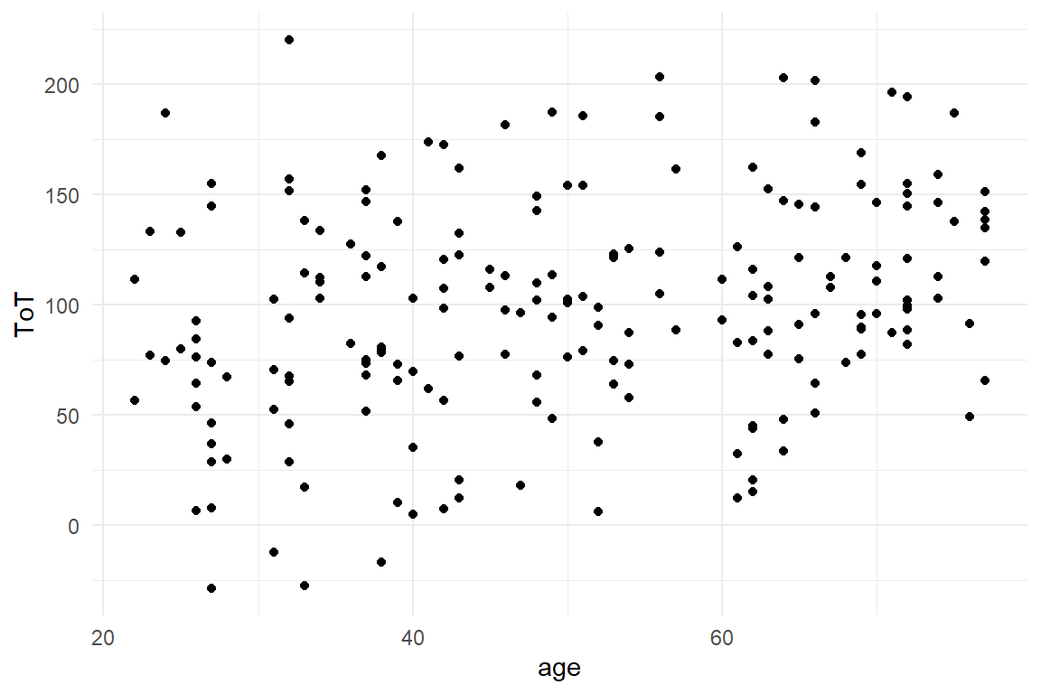
Figure 2.2: Scatterplot showing the assiciation between age and ToT
Let’s take a look at the elements of the command chain: The first two lines pipe the data frame into the ggplot engine.
BAB1 %>%
  ggplot()
At that moment, the ggplot engine “knows” which variables the data frame
contains and hence are available for the plot. It does not yet know,
which variables are being used, and how. The next step is, usually, to
consider a basic (there exist more than 30) geometry and put it on a
layer. The scatter plot geometry of ggplot is geom_point:
BAB1 %>%
  ggplot() +
  geom_point()
The last step is the aesthetic mapping, which tells ggplot the variables to use and how to map them to visual properties of the geometry. The basic properties of points in a coordinate system are the x and y-positions:
BAB1 %>%
  ggplot(aes(x = age, y = ToT)) +
  geom_point()
The function aes creates a mapping where the aesthetics per variable
are given. When call aes directly, we see that it really is just a table.
aes(x = age, y = ToT)## Aesthetic mapping:
## * `x` -> `age`
## * `y` -> `ToT`One tiny detail in the above chain has not yet been explained: the +.
When choosing the geometry, you actually add a layer to the plot. This
is, of course, not the literal mathematical sum. Technically, what the
author of the ggplot2 package did, was to overload the + operator. A
large set of ggplot functions can be combined in a myriad of ways, just
using +. The overloaded + in ggplot is a brilliant analogy: you can
infinitely chain ggplot functions, like you can create long sums. You
can store ggplot object and later modify it by adding functions. The
analogy has its limits, though: other than sums, order matters in ggplot
combinations: the first in the chain is always ggplot and layers are
drawn upon each other.
Let’s move on with a slightly different situation that will result in a different geometry. Say, we are interested in the distribution of the time-on-task measures under the two designs. We need a geometry, that visualizes the distribution of quantitative variables split by a grouping variable, factor. The box plot does the job (Figure 2.3) :
BAB1 %>%
  ggplot(aes(x = Design, y = ToT)) +
  geom_boxplot()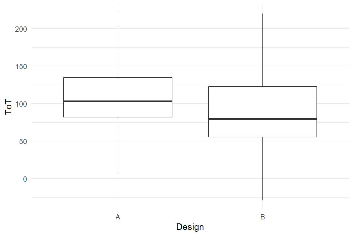
Figure 2.3: A boxplot
The box plot maps ToT to y (again). The factor Design is represented as a split on the x-axis. Interestingly, the box plot does not represent the data as raw as in the scatter plot example. The geometry actually performs an analysis on ToT, which produces five statistics: min, first quartile, median, third quartile and max. These statistics define the vertical positions of bars and end points.
Now, we combine all three variables in one plot: how does the
association between ToT and age differ by design? As we have two
quantitative variables, we stay with the scatter plot for now. As we
intend to separate the groups, we need a property of points to
distinguish them. Points offer several additional aesthetics, such as
color, size and shape. We choose color, and add it to the aesthetic
mapping by aes (Figure 2.4)
. Note, that it does not matter whether you use the
British or American way of writing (colour vs. color).
BAB1 %>%
  ggplot(aes(x = age, y = ToT, color = Design)) +
  geom_point()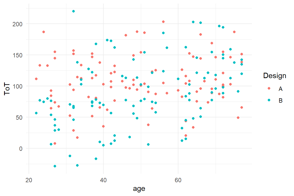
Figure 2.4: A grouped scatterplot
Now, we can distinguish the groups visually, but there is too much
clutter to discover any relation. With the box plot we saw that some
geometries do not represent the raw data, but summaries (statistics) of
data. For scatter plots, a geometry that does the job of summarizing the
trend is geom_smooth. This geometry summarizes a cloud of points by
drawing a LOESS-smooth line through it. Note how the color mapping is
applied to all geometry layers (Figure 2.5)
.
BAB1 %>%
  ggplot(aes(x = age, y = ToT, color = Design)) +
  geom_point() +
  geom_smooth()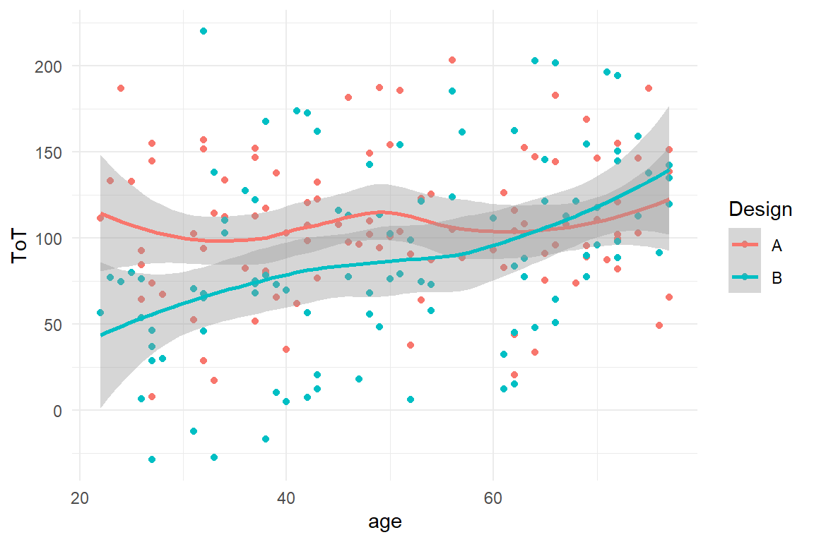
Figure 2.5: A scatterplot with smoothed lines
We see a highly interesting pattern: the association between age and ToT follows two slightly different mirrored sigmoid curves.
Now that we have represented three variables with properties of geometries, what if we wanted to add a fourth one, say education level? Formally, we could use another aesthetic, say shape of points, to represent it. You can easily imagine that this would no longer result in a clear visual figure. For situations, where there are many factors, or factors with many levels, it is impossible to reasonably represent them in one plot. The alternative is to use facetting. A facet splits the data by a grouping variable and creates one single plot for every group (Figure 2.6).
BAB1 %>%
  ggplot(aes(x = age, y = ToT, color = Design)) +
  geom_point() +
  geom_smooth() +
  facet_grid(Education ~ .)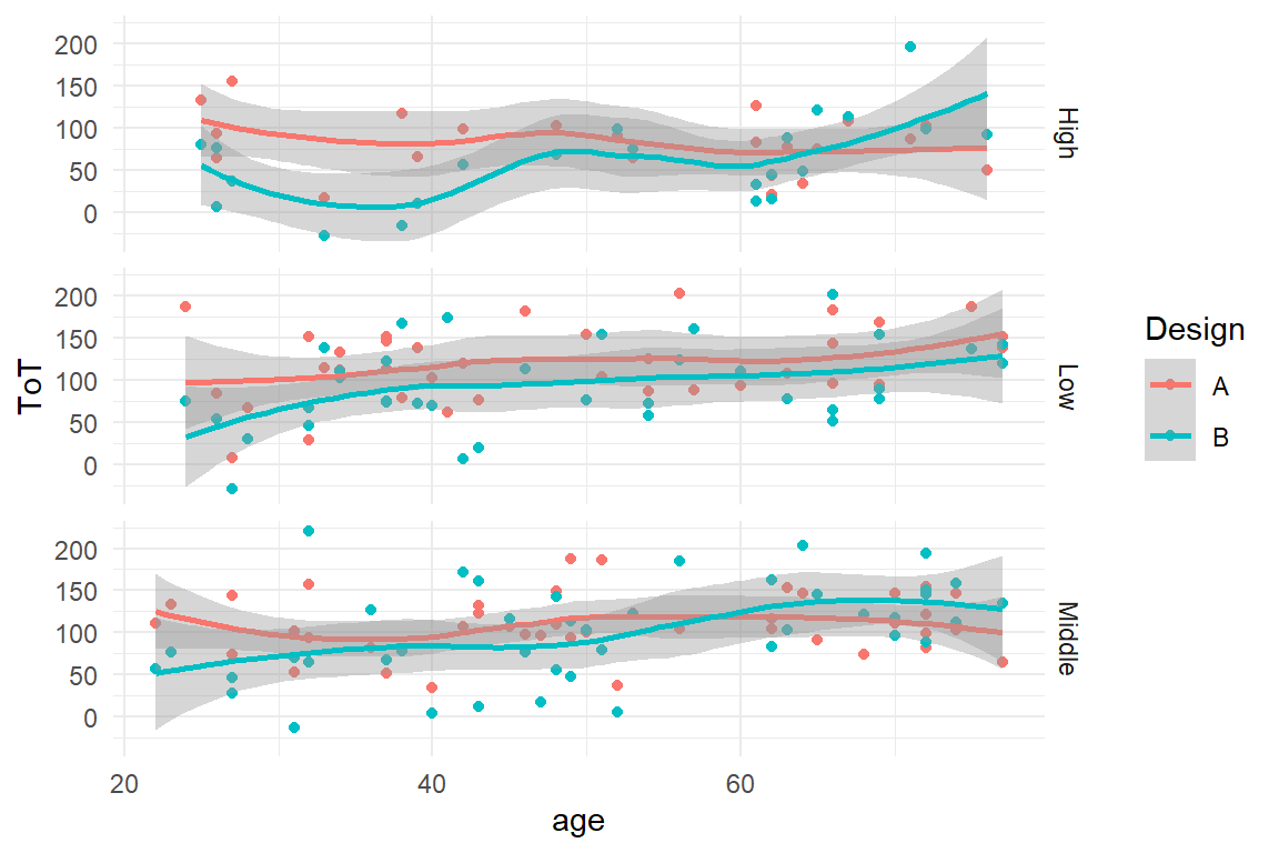
Figure 2.6: With facets groups can be distinguished
See, how the facet_grid command takes a formula, instead of just a
variable name. This makes faceting the primary choice for
highly-dimensional situations. For example, we may also choose to
represent both factors, Design and education by facets (Figure 2.7)
:
BAB1 %>%
  ggplot(aes(x = age, y = ToT)) +
  geom_point() +
  geom_smooth() +
  facet_grid(Education ~ Design)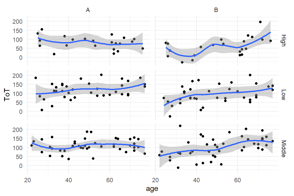
Figure 2.7: Facetting by two factors (or more) results in a grid
Note how the color aesthetic, although unnecessary, is kept. It is possible to map several aesthetics (or facets) to one variable, but not vice versa.
2.2.11 Fitting regression models
Above we have seen examples of functions that boil down a vector to a
single statistic, like the mean. R has several functions that summarize
data in a more complex way. One function with a wide range of
applications is the lm command, that applies regression models to data
(provided as data frames).
In the following, we will use another simulated data frame Exp to
demonstrate linear models. To make this more interesting, we simulate
Exp in a slightly advanced way, with quantitative associations between
variables. Note how the expected value \(\mu\) is created by drawing on
the variables Condition and age. The last step adds (somewhat)
realistic noise to the measures, by drawing from the normal distribution
with a mean of \(mu\).
N_Obs <- 20
set.seed(42)
Exp <-
  tibble(
    Obs = 1:N_Obs,
    Condition = rep(
      c("Experimental", "Control"),
      N_Obs / 2
    ),
    age = runif(N_Obs, 18, 35),
    mu = 200 + (Condition == "Control") * 50 + age * 1,
    outcome = rnorm(N_Obs, mu, 10)
  )
The experiment involves two groups, which in classic statistics would
clearly point to what is commonly referred to as ANOVA. As it will
turn out in 4.3.1, old-fashioned ANOVA can be replaced by a rather
simple regression model, that I call comparison of groups model (CGM).
The estimation of regression models is done by a regression engine,
which basically is a (very powerful) R command. The specification for
any regression model is given in R’s formula language. Learning this
formula language is key to unleashing the power of regression models in
R. We can perform a CGM on the data frame Exp using the regression
engine stan_glm. The desired model estimates the effect of Condition
on outcome. This produces a regression object that contains an
abundance of information, much of it is of little interest for now. (A
piece of information, that it does not contain is F-statistics and
p-values; and that is why it is not an ANOVA, strictly speaking!) The
foremost question is how strong the difference between the groups is.
The clu command extracts the parameter estimates from the model to
answer the question (Table 2.16).
M_1 <-
  stan_glm(outcome ~ Condition,
    data = Exp
)clu(M_1)| parameter | fixef | center | lower | upper |
|---|---|---|---|---|
| Intercept | Intercept | 275.6 | 264.2 | 286.0 |
| ConditionExperimental | ConditionExperimental | -47.8 | -62.5 | -31.9 |
| sigma_resid | 16.8 | 12.3 | 24.5 |
Another classic model is linear regression, where outcome is predicted
by a metric variable, say age. Estimating such a model with stan_glm looks like this, and Table 2.17 shows the estimated parameters.
M_2 <-
  stan_glm(outcome ~ age,
    data = Exp
)clu(M_2)| parameter | fixef | center | lower | upper |
|---|---|---|---|---|
| Intercept | Intercept | 220.29 | 132.1 | 306.69 |
| age | age | 1.09 | -1.9 | 4.17 |
| sigma_resid | 30.11 | 22.3 | 43.43 |
If you are interested in both at the same time, you can combine that in one model by the following formula. As a result, Table 2.18 now has three parameters, two of which are coefficients (fixef).
M_3 <-
  stan_glm(outcome ~ Condition + age,
    data = Exp
)clu(M_3)| parameter | fixef | center | lower | upper |
|---|---|---|---|---|
| Intercept | Intercept | 220.1 | 178.744 | 261.79 |
| ConditionExperimental | ConditionExperimental | -50.4 | -63.321 | -37.06 |
| age | age | 2.0 | 0.551 | 3.45 |
| sigma_resid | 14.2 | 10.309 | 20.87 |
A statistical model has several components, for example the coefficients
and residuals. Models are complex objects, from which a variety of
inferences can be made. For example, the coefficient estimates can be
extracted and used for prediction. This is what fixef() does in the
above code.
A number of functions can be used to extract certain aspects of the model. For example:
fixef(model)extracts the linear coefficientsresiduals(model)extracts the measurement errorspredict(model)extracts the expected values
These will all be covered in later chapters.
2.2.12 Knitting statistical reports
As you have seen throughout this chapter, with R you can effectively manage data, create impressively expressive graphics and conveniently estimate statistical models. Then usually comes the painful moment where all this needs to be assembled into a neat report. With R and Rstudio it has never been easier than that. In fact, complete books have been written in R, like the one you are reading.
A minimal statistical report contains four elements:
- a recap of the research question
- description of how the statistical model relates to the research question
- a few figures or tables that answers the research question
- an explanation of the results
Of these four elements, three are pure text. For a minimal report it is a fairly convenient to use a word processor software for the text, craft the figure in R and copy it. One problem with this approach is that a scrunitable statistical report contains at least the following additional elements:
- procedures of data preparation (sources, transformations, variable names, outlier removal)
- data exploration (ranges of variables, outlier discovery, visualizing associations, etc.)
- model estimation (formula specification, convergence checks)
- model criticism (normality of residuals, etc.)
In advanced statistical workflows this is then multiplied by the number of models, an iterative selection process. Because it is easy to lie with statistics, these elements are needed as to build a fundament of credibility. Full transparency is achieved, when another researcher can exactly reproduce all steps of the original analysis. It is obvious that the easiest way to achieve this, is to hand over the full R script.
The most user-friendly way to achieve both, a good looking report and full transparency, is to write a document that contains all before mentioned: text, graphics, tables and R code. In the R environment such mixed documents can be written in the markdown/knitr framework.
Markdown implements a simple markup language, with that you can typset simple, structured texts in a plain ASCII editor. Later in the workflow, such a markup document is transformed into one of various output formats, that are rendered by the respective programs, such as Microsoft Word or an HTML browser.
A minimal statistical report in markdown
The above text is an alternation of markup text and chunks, those
weirdly enclosed pieces of R code. While the text is static, the chunks
are processed by the knitr engine, evaluating the enclosed R code and
knitting the output into a document. Very conveniently, when the output
is a figure, it will be inserted into the document right away. The
kable command from the knitr package, in turn, produces neatly
rendered tables from data frame objects. By default, the R code is
shown, too, but that can be customized.
The minimal workflow for statistical reporting with knitr is as follows:
- Use markdown right away, covering all steps of your data analysis, i.e. a scrutable report. You may even start writing when only one part of your data gathering is completed, because due to the dynamic chunks, updating the report when new data arrives is just a button click away.
- When the data analysis is complete, compile the scrutable report to Word format
- Extract the passages, figures and tables for a minimal statistical report. This is your results section.
- provide the scrutable report as appendix or supplementary material
In the notion of this chapter, this is just to get you started and knitr is so tightly integrated with the Rstudio environment that I don’t even bother to explain the commands for knitting a document. Once acquainted with the basics, markdown provides a few additional markup tokens, like footnotes, hyperlinks or including images. The customization options and addons for knitr are almost endless and various interesting addons are available, just to mention two:
- The bookdown package provides an infrastructure for writing and publishing longer reports and books.
- With the shiny package one can add dynamic widgets to HTML reports. Think of a case, where your statistical model is more complicated than a linear regression line or a few group means, say you are estimating a polynomial model or a learning curve. Then, with a simple shiny app, you can enable your readers to understand the model by playful exploration
2.3 Further reading
1.R for Data Science is a book co-authored by Hadley “Tidy” Wickham. 1. The Grammar of Graphics, (Leland Wilkinson 2005) is the formal framework for the ggplot engine. 1.ggplot2 Version of Figures in “25 Recipes for Getting Started with R” for readers who are familiar with the legacy plotting commands in R. 1. Introduction to dplyr for Faster Data Manipulation in R introduces dplyr, the next generation R interface for data manipulation, which is used extensively in this book. 1. Quick-R is a comprehensive introduction to many common statistical techniques with R. 1. Code as manuscript features a small set of lessons with code examples, assignments and further resources. For if you are in a haste. 1. bookdown: Authoring Books and Technical Documents with R Markdown fully unleashes the power of knitr for writing and publishing longer reports and books. 1. Rstudio Cheatsheets a growing collection of cheatsheets for tidy R and more.