6 Multilevel models
In the previous chapters we have seen several examples of conditional effects: groups of users responding differently to design conditions, such as font size, noise and emerging technology. Dealing with differential design effects seems straight forward: identify the relevant property, record it and add an conditional effect to the model.
Identifying user properties that matter requires careful review of past research or deep theorizing, and even then it remains guesswork. Presumably, hundreds of studies attempted to explain differences in usage patterns or performance by all sorts of psychological predictors, with often limited results. That is a big problem in design research, as variation in performance can be huge and good predictors are urgently needed. Identifying the mental origins of being fast versus slow, or motivated versus bored, is extremely useful to improve the design of systems to be more inclusive or engaging.
As we will see in this chapter, individual differences can be accounted for and measured accurately without any theory of individual differences. For researchers trained in experimental social sciences it may require a bit of getting used to theory-free reasoning about effects, as it is always tempting to ask for the why. But in applied evaluation studies, what we often really need to know is by how much users vary. The key to measuring variation in a population is to create models that operate on the level of participants, in addition to the population level, for example.
- on population level, users prefer design B over A on average (\(\beta_1 = 20\))
- on the participant-level, participant \(i\) preferred B over A (\(\beta_{1i} = 20\)), \(j\) preferred A over B (\(\beta_{1j} = -5\)), +
When adding a participant-level effects, we still operate with coefficients, but in contrast to single-level linear models, every participant gets their own coefficient (\(\beta_{1\cdot}\)). The key to estimating individual parameters is simply to regard participant (Part) a grouping variable on its own, and introduce it as a factor.
The subsequent two sections introduce the basics of estimating multi-level linear models, first introducing intercept-only participant-level effects 6.1 and then slope (or group difference) effects 6.2. Typically, fixed and random effects appear together in a linear multi-level model. It depends on the research question whether the researcher capitalizes on the average outcome, the variation in the population or participant-level effects.
The participant-level is really just the factor and once it is regarded alongside the population level, a model is multi-level. However, in multi-level linear modelling we usually use a different type of factor, for the particpant level. The additional idea is that the levels of the factor, hence the individuals, are part of a population. The consequences of this perspective, will be discussed in 6.7: a population is a set of entities that vary to some extent but also clump around a typical value. And that is precisely what random effects do: levels are drawn from an overarching distribution, usually the Gaussian. This distribution is estimated simultaneously to the individual parameters (\(\beta_{1\cdot}\)), which has advantages. We will return to a more fundamental research case, the Uncanny Valley, and examine the universality of this strange effect 6.4.
Once it is clear what the concept of random effects means for studying participant behaviour, we will see that it transfers with grace to non-human populations, such as designs, teams or questionnaire items. Three sections introduce multi-population multi-level models: In 6.5 we will use a random effects model with four populations and compare their relative contribution to overall variance in performance. Section @ref(re_nested) will show how multiple levels can form a hierarchy and in 6.8 we will see that multi-level models can be employed the development of psychometrics tests, that apply for people. Finally, we will see how to treat tests to compare designs, for which I will coin the term design-o-metrics 6.8.4.
6.1 The Human Factor: Intercept random effects
Design science fundamentally deals with interaction between systems and humans. Every measure we take in a design study is an encounter of an individual with a system. As people differ in many aspects, it is likely that people differ in how they use and perform with a system. In the previous chapter we have already dealt with differences between users: in the BrowsingAB case, we compared two designs in how inclusive they are with respect to elderly users. Such a research question seeks for a definitive answer on what truly causes variation in performance. Years of age is a standard demographic variable and in experimental studies it can be collected without hassle. If we start from deeper theoretical considerations than that, for example, we suspect a certain personality trait to play a significant role, this can become more effort. Perhaps, you need a 24-item scale to measure the construct, perhaps you first have to translate this particular questionnaire into three different languages, and perhaps you have to first invent and evaluate a scale. In my experience, personality scales rarely explain much of the variation we see in performance. It may be interesting to catch some small signals for the purpose of testing theories, but for applied design research it is more important to quantify the performance variation within a population, rather than explaining it.
At first, one might incorrectly think that a grand mean model would do, take \(\beta_0\) as the population mean and \(\sigma_\epsilon\) as a measure for individual variation. The mistake is that the residuals collect all random variations sources, not just variance between individuals, in particular residuals are themselves composed of:
- inter-individual variation
- intra-individual variation, e.g. by different levels of energy over the day
- variations in situations, e.g. responsiveness of the website
- inaccuracy of measures, e.g. misunderstanding a questionnaire item
What is needed, is a way to separate the variation of participants from the rest? Reconsider the principles of model formulations: the structural part captures what is repeatable, what does not repeat goes to the random term. This principle can be turned around: If you want to pull a factor from the random part to the structural part, you need repetition. For estimating users’ individual performance level, all that is needed is repeated measures.
In the IPump study we have collected performance data of 25 nurses, operating a novel interface for a syringe infusion pump. Altogether, every nurse completed a set of eight tasks three times. Medical devices are high-risk systems where a single fault can cost a life, which makes it a requirement that user performance is on a uniformly high level. We start the investigation with the global question (Table 6.1):
What is the average ToT in the population?
attach(IPump)D_Novel %>%
summarize(mean_Pop = mean(ToT)) | mean_Pop |
|---|
| 16 |
The answer is just one number and does not refer to any individuals in the population. This is called the population-level estimate or fixed effect estimate. The following question is similar, but here one average is taken for every participant. We call such a summary participant-level (Table 6.2).
What is the average ToT of individual participants?
D_Novel %>%
  group_by(Part) %>%
  summarize(mean_Part = mean(ToT)) %>%
sample_n(5) | Part | mean_Part |
|---|---|
| 3 | 14.14 |
| 10 | 14.18 |
| 5 | 15.97 |
| 2 | 16.70 |
| 7 | 9.24 |
Such a grouped summary can be useful for situations where we want to directly compare individuals, like in performance tests. In experimental research, individual participants are of lesser interest, as they are exchangeable entities. What matters is the total variation within the sample, representing the population of users. Once we have participant-level effects, the amount of variation can be summarized by the standard deviation (Table 6.3):
D_Novel %>%
  group_by(Part) %>%
  summarize(mean_Part = mean(ToT)) %>%
  ungroup() %>%
summarize(sd_Part = var(mean_Part)) | sd_Part |
|---|
| 13.8 |
Generally, these are the three types of parameters in multi-level models: the population-level estimate (commonly called fixed effects), the participant-level estimates (random effects) and the participant-level variation.
Obviously, the variable Part is key to build such a model. This variable groups observations by participant identity and, formally, is a plain factor. A naive approach to multi-level modeling would be to estimate an AGM, like ToT ~ 0 + Part, grab the center estimates and compute the standard deviation. What sets a truly multi-level apart is that population-level effects, participant-level effects and variation are contained in one model and are estimated simultaneously. Random effects are really just factors with one level per participant. The only difference to a fixed effects factor is that the levels are assumed to follow a Gaussian distribution. This will further be explained in section 6.7.
For the IPump study we can formulate a GMM model with participant-level random effect \(\beta_{p0}\) as follows:
\[ \begin{aligned} \mu_i &= \beta_0 + x_p\beta_{0p}\\ \beta_{p0} &\sim \textrm{Gaus}(0, \sigma_{p0})\\ y_i &\sim \textrm{Gaus}(\mu_i, \sigma_\epsilon) \end{aligned} \]
There will be as many parameters \(\beta_{0p}\), as there were participants in the sample, and they have all become part of the structural part. The second term describes the distribution of the participant-level group means. And finally, there is the usual random term. Before we examine further features of the model, let’s run it. In the package rstanarm, the command stan_glmer is dedicated to estimating multi-level models with the extended formula syntax.
However, I will now introduce another Bayesian engine and use it from here on. The Brms package provides the Brm engine, which is invoked by the command brm(). This engine covers all models that can be estimated with stan_glm or stan_glmer and it uses the precise same syntax. All models estimated in this chapter, should also work with stan_glmer. However, Brms supports an even broader set of models, some of which we will encounter in chapter 7.
The only downside of Brms is that it has to compile the model, preceding the estimation. For simple models, as in the previous chapter, the chains are running very quickly, and the extra step of compilation creates much overhead. For the models in this chapter, the chains run much slower, such that compilation time becomes almost negligible.
Both engines Brms and Rstanarm differ a lot in how they present the results. The Bayr package provides a consistent interface to extract information from model objects of both engines.
attach(IPump)M_hf <- brm(ToT ~ 1 + (1 | Part), data = D_Novel)
P_hf <- posterior(M_hf)The posterior of a multi-level model contains three types of variables (and the standard error)
- the fixed effect captures the population average (Intercept)
- random effects capture how individual participants deviate from the population mean
- random factor variation (or group effects) captures the overall variation in the population.
With the bayr package these parameters can be extracted using the respective commands (Table 6.4, 6.5 and 6.6):
fixef(P_hf)| model | type | fixef | center | lower | upper |
|---|---|---|---|---|---|
| M_hf | fixef | Intercept | 16 | 14.4 | 17.5 |
ranef(P_hf) %>% sample_n(5)| re_entity | center | lower | upper |
|---|---|---|---|
| 9 | 0.402 | -2.19 | 4.50 |
| 13 | 0.246 | -2.59 | 4.33 |
| 23 | -0.440 | -4.53 | 1.99 |
| 21 | -0.297 | -4.29 | 2.16 |
| 16 | -0.019 | -3.26 | 3.22 |
grpef(P_hf)| model | type | fixef | re_factor | center | lower | upper |
|---|---|---|---|---|---|---|
| M_hf | grpef | Intercept | Part | 1.53 | 0.079 | 3.73 |
Random effects are factors and enter the model formula just as linear terms. To indicate that to the regression engine, a dedicated syntax is used in the model formula (recall that 1 represents the intercept parameter):
(1|Part)
In probability theory expressions, such as the famous Bayes theorem, the | symbol means that something to the left is conditional on something to the right. Random effects can be read as such conditional effects. Left of the | is the fixed effect that is conditional on (i.e. varies by) the factor to the right. In the simplest form the varying effect is the intercept and in the case here could be spoken of as:
Average ToT, conditional on the participant
Speaking of factors: So far, we have used treatment contrasts as lot for population-level factors, which represent the difference towards a reference level. If random effects were coded as treatment effects, we would have one absolute score for the first participants (reference group). All other average scores, we would express as differences to the reference participant. This seems odd and, indeed, has two disadvantages: first, whom are we to select as the reference participant? The choice would be arbitrary, unless we wanted to compare brain sizes against the grey matter of Albert Einstein, perhaps. Second, most of the time the researcher is after the factor variation rather than differences between any two individuals, which is inconvenient to compute from treatment contrasts.
The solution is to use a different contrast coding for random factors: deviation contrasts represent the individual effects as difference (\(\delta\)) towards the population mean. As the population mean is represented by the respective fixed effect, we can compute the absolute individual predictions by adding the fixed effect to the random effect. The results are shown in Figure 6.1.
tibble(mu_i = ranef(P_hf)$center +
  fixef(P_hf)$center) %>%
  ggplot(aes(x = mu_i)) +
  geom_histogram()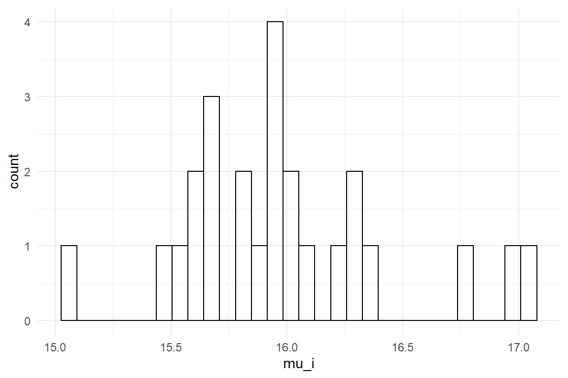
Figure 6.1: Absolute random effect scores
Note that first two lines in the above code only work correctly if there is just one population-level effect (i.e. a GMM). Package Bayr contains the general re_score to produce absolute random effects scores. This happens on the level of MCMC samples, from which CLUs can extracted, such as (Table 6.7).
re_scores(P_hf) %>%
  clu() %>%
sample_n(8)| parameter | re_entity | center | lower | upper |
|---|---|---|---|---|
| r_Part[21,Intercept] | 21 | 15.5 | 11.6 | 18.4 |
| r_Part[22,Intercept] | 22 | 15.5 | 11.4 | 18.4 |
| r_Part[1,Intercept] | 1 | 17.1 | 14.5 | 22.4 |
| r_Part[3,Intercept] | 3 | 15.7 | 11.9 | 18.8 |
| r_Part[13,Intercept] | 13 | 16.3 | 13.2 | 20.3 |
| r_Part[20,Intercept] | 20 | 16.4 | 13.7 | 20.3 |
| r_Part[10,Intercept] | 10 | 15.7 | 12.0 | 18.9 |
| r_Part[12,Intercept] | 12 | 16.4 | 13.4 | 20.4 |
Finally, we can assess the initial question: are individual differences a significant component of all variation in the experiment? Assessing the impact of variation is not as straight-forward as with fixed effects. Two useful heuristics are to compare group-level variation to the fixed effects estimate (Intercept) and against the standard error:
P_hf %>%
  filter(type %in% c("grpef", "disp", "fixef")) %>%
clu()| parameter | fixef | re_factor | center | lower | upper |
|---|---|---|---|---|---|
| b_Intercept | Intercept | 15.96 | 14.423 | 17.46 | |
| sd_Part__Intercept | Intercept | Part | 1.53 | 0.079 | 3.73 |
| sigma | 16.39 | 15.488 | 17.39 |
The variation due to individual differences is an order of magnitude smaller than the Intercept, as well as the standard error. This lets us conclude that the novel interface works pretty much the same for every participant. If we are looking for relevant sources of variation, we have to look elsewhere. (As we have seen in 4.3.5, the main source of variation is learning.)
6.2 Multi-level linear regression: variance in change
So far, we have dealt with Intercept random effects that capture the gross differences between participants of a sample. We introduced these random effects as conditional effects like: “average performance depends on what person you are looking at.” However, most research questions rather regard differences between conditions.
With slope random effects we can represent individual changes in performance. For an illustration of slope random effects, we take a look at a data set that ships with package Lme4 (which provides a non-Bayesian engine for multi-level models). 18 participants underwent sleep deprivation on ten successive days and the average reaction time on a set of tests has been recorded per day and participant. The research question is: what is the effect of sleep deprivation on reaction time and, again, this question can be asked on population level and participant level.
The participant-level plots in Figure 6.2 shows the individual relationships between days of deprivation and reaction time. For most participants a positive linear association seems to be a good approximation, so we can go with a straight linear regression model, rather than an ordered factor model. One noticeable exception is the curve of participant 352, which is fairly linear, but reaction times get shorter with sleep deprivation. What would be the most likely explanation? Perhaps, 352 is a cheater, who slept secretly and improved by gaining experience with the task. That would explain the outstanding performance the participant reaches.
attach(Sleepstudy)D_slpstd %>%
ggplot(aes(x = days, y = RT)) +
facet_wrap(~Part) +
geom_point() +
geom_smooth(se = F, aes(color = "LOESS")) +
geom_smooth(se = F, method = "lm", aes(color = "Linear model")) +
labs(color = "Smoothing function") +
theme(legend.position = c(0.8, 0.1)) # !del+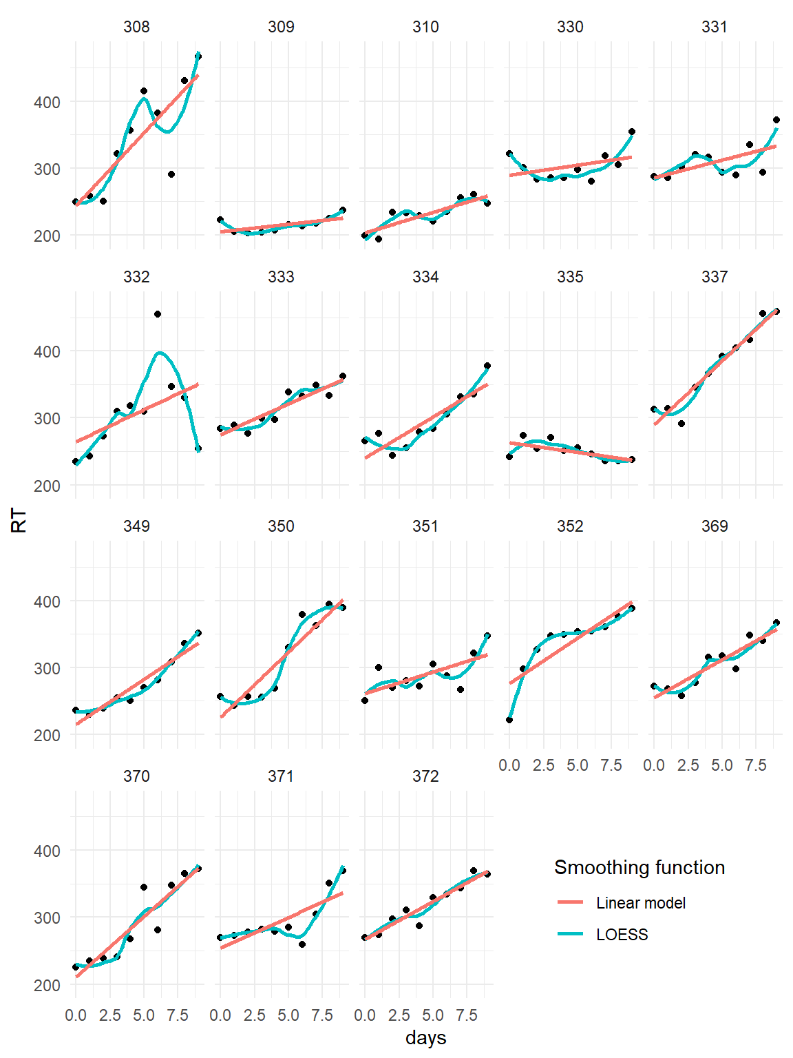
Figure 6.2: Participant-level association between sleep deprivation and RT
A more compact way of plotting multi-level slopes is the spaghetti plot below. By superimposing the population level effect, we can clearly see that participants vary in how sleep deprivation delays the reactions.
D_slpstd %>%
  ggplot(aes(
    x = days,
    y = RT,
    group = Part
  )) +
  geom_smooth(aes(color = "participant"),
    size = .5, se = F, method = "lm"
  ) +
  geom_smooth(aes(group = 1, color = "population"),
    size = 2, se = F, method = "lm"
  ) +
  labs(color = "Level of Effect")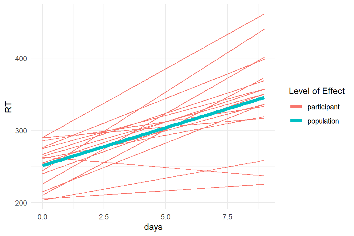
Figure 6.3: (Uncooked) Spaghetti plot showing population and participant-level effects
For a single level model, the formula would be RT ~ 1 + days, with the intercept being RT at day Zero and the coefficient days representing the change per day of sleep deprivation. The multi-level formula retains the population level and adds the participant-level term as a conditional statement: again, the effect depends on whom you are looking at.
RT ~ 1 + days + (1 + days|Part)
Remember to always put complex random effects into brackets, because the + operator has higher precedence than |. We estimate the multi-level model using the Rstanarm engine.
M_slpsty_1 <- brm(RT ~ 1 + days + (1 + days | Part),
  data = D_slpstd,
  iter = 2000
)
Again, we could use the commands fixef, ranef and grpef to extract the parameters, but Bayr also provides a specialized command for multi-level tables, as Table 6.9: fixef_ml extracts the population-level estimates in CLU form and adds the participant-level standard deviation. The overall penalty for sleep deprivation is around ten milliseconds per day, with a 95% CI ranging from 7ms to 14ms. At the same time, the participant-level standard deviation is around 6.5ms, which is considerable. One can conclude that people vary a lot in how sleep deprivation effects their alertness. Figure 6.4 shows a caterpillar plot of the slope random effects, ordered by the center estimate.
fixef_ml(M_slpsty_1)| fixef | center | lower | upper | SD_Part |
|---|---|---|---|---|
| Intercept | 251.2 | 237.17 | 265.8 | 26.1 |
| days | 10.5 | 7.01 | 13.8 | 6.4 |
ranef(M_slpsty_1) %>%
  filter(fixef == "days") %>%
  mutate(Part_ord = rank(center)) %>%
  ggplot(aes(x = Part_ord, ymin = lower, y = center, ymax = upper)) +
  geom_crossbar() +
  labs(y = "diff RT")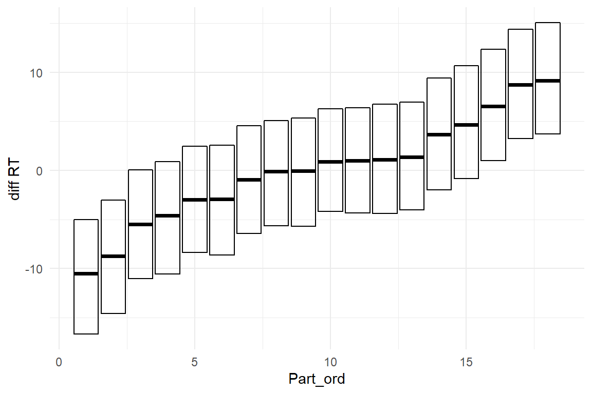
Figure 6.4: Caterpillar plot showing individual absolute scores for effect of one day of sleep deprivation
The multi-level regression model is mathematically specified as follows. Note how random coefficients \(\beta_{.(Part)}\) are drawn from a Gaussian distribution with their own standard deviation, very similar to the errors \(\epsilon_i\).
\[ \begin{aligned} y_i &= \mu_i + \epsilon_i\\ \mu_i &= \beta_0 + \beta_{0(Part)} + x_1 \beta_1 + x_{1}\beta_{1(Part)}\\ \beta_{0(Part))} &\sim \textrm{Gaus}(0,\sigma_{0(Part)})\\ \beta_{1(Part))} &\sim \textrm{Gaus}(0,\sigma_{1(Part)})\\ \epsilon_i &= \textrm{Gaus}(0, \sigma_\epsilon) \end{aligned} \]
The second line can also be written as:
\[ \mu_i = \beta_0 + \beta_{0(Part)} + x_1 (\beta_1 + \beta_{1(Part)}) \]
This underlines that random coefficients are additive correction terms to the population-level effect, which is what ranef reports. Sometimes, it is useful to look at the total scores per participant. In package Bayr, the command re_scores computes absolute scores on the level of the posterior distribution. The following plot uses this command and plots two distributions: The participant-level variation in RT at Day 1 (Intercept) and after twenty nights* of sleep interruption, (assuming that the association is linear beyond the observed range). Figure 6.5 shows the participant-level trajectories. We learn from it, that long-term sleep interruption creates a huge variance. If you design for a population where long-term sleep deprivation occurs, such as parents or doctors, and reaction time is critical, the worst case can be much, much worse than the average.
posterior(M_slpsty_1) %>%
  re_scores() %>%
  clu() %>%
  select(re_entity, fixef, center) %>%
  pivot_wider(names_from = fixef, values_from = center) %>%
  ggplot() +
  geom_abline(aes(
    intercept = Intercept,
    slope = days
  )) +
  xlim(0, 20) +
  ylim(0, 700)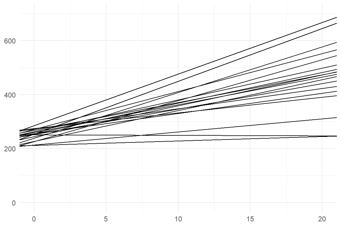
Figure 6.5: Sleep deprivation projected
6.3 Thinking multi-level
There is a lot of confusion about the type of models that we deal with in this chapter. They have also been called hierarchical models or mixed effects models. The “mixed” stands for a mixture of so called fixed effects and random effects. The problem is: if you start by understanding what fixed effects and random effects are, confusion is programmed, not only because there exist several very different definitions.
In fact, it does not matter so much whether an estimate is a fixed effect or random effect. As we will see, you can construct a multi-level model by using just plain descriptive summaries. What matters is that a model contains estimates on population level and on participant level. The benefit is, that a multi-level model can answer the same question for the population as a whole and for every single participant.
For entering the world of multi-level modeling, we do not need fancy tools. More important is to start thinking multi-level. In the following, I will introduce the basic ideas of multi-level modeling at the example of the IPump case. The idea is simple: A statistical model is developed on the population level and then we “pull it down” to the participant level.
In the IPump case, a novel syringe infusion pump design has been tested against a legacy design by letting trained nurses complete a series of eight tasks. Every nurse repeated the series three times on both designs. Time-on-task was measured and the primary research question is:
Does the novel design lead to faster execution of tasks?
attach(IPump)To answer this question, we can compare the two group means using a basic CGM (Table 6.10)
M_cgm <- stan_glm(ToT ~ 1 + Design,
  data = D_pumps
)fixef(M_cgm)| fixef | center | lower | upper |
|---|---|---|---|
| Intercept | 27.9 | 25.9 | 29.76 |
| DesignNovel | -11.8 | -14.5 | -9.17 |
This model is a single-level model. It takes all observations as “from the population” and estimates the means in both groups. It further predicts that with this population of users, the novel design is faster on average, that means taking the whole population into account, (and forgetting about individuals).
An average benefit sounds promising, but we should be clear what it precisely means, or better what it does not mean: That there is a benefit for the population does not imply, that every individual user has precisely that benefit. It does not even imply that every user has a benefit at all. In extreme case, a small subgroup could be negatively affected by the novel design, but this could still result in a positive result on average. In the evaluation of high-risk devices like infusion pumps concerns about individual performance are real and this is why we designed the study with within-subject conditions, which allows to estimate the same model on population level and participant level. The following code produces a multi-level descriptive model. First, a summary on participant level is calculated, then it is summarized to obtain the population level. By putting both summaries into one figure, we are doing a multi-level analysis.
T_Part <-
  D_pumps %>%
  group_by(Part, Design) %>%
  summarize(mean_Part = mean(ToT))

T_Pop <-
  T_Part %>%
  group_by(Design) %>%
summarize(mean_Pop = mean(mean_Part))gridExtra::grid.arrange(
nrow = 2,
T_Pop %>%
ggplot(aes(
x = Design, group = NA,
y = mean_Pop
)) +
geom_point() +
geom_line() +
ggtitle("Population-level model (average benefits)") +
ylim(0, 60),
T_Part %>%
ggplot(aes(
x = Design,
y = mean_Part,
group = Part, label = Part
)) +
geom_line() +
ggrepel::geom_label_repel(size = 3, alpha = .5) +
ggtitle("Participant-level model (individual benefits)") +
ylim(0, 60)
)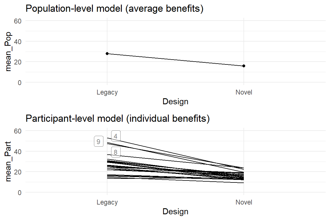
Figure 6.6: Exploratory multi-level plot of population-level and participant-level change
Note
- how with
gridExtra::grid.arrange()we can multiple plots into a grid, which is more flexible than using facetting - that
ggrepel::geom_label_repelproduces non-overlapping labels in plots
Figure 6.6 is a multi-level plot, as it shows the same effect on two different levels alongside. In this case, the participant-level plot confirms that the trend of the population-level effects is representative. Most worries about the novel design are removed, with the one exception of participant 3, all users had net benefit from using the novel design and we can call the novel design universally better. In addition, some users (4, 8 and 9) seem to have experienced catastrophes with the legacy design, but their difficulties disappear when they switch to the novel design.
If you look again at the participant-level spaghetti plot (They are uncooked!) and find it similar to what you have seen before, you are right: This is an design-by-participant conditional plot. Recall, that conditional effects represent the change of outcome, depending on another factor. In this multi-level model, this second factor simply Part(icipant). That suggests that it is well within reach of plain linear models to estimate design-by-participant conditional effects. Just for the purpose of demonstration, we can estimate a population level model, conditioning the design effect on participants. Ideally, we would use a parametrization giving us separate Intercept and DesignNovel effects per participant, but the formula interface is not flexible enough and we would have to work with dummy variable expansion. Since this is just a demonstration before we move on to the multi-level formula extensions, I use an AMM instead. A plain linear model can only hold one level at a time, which is why we have to estimate the two separate models for population and participant levels. Then we combine the posterior objects, extract the CLU table and plot the center estimates in Figure 6.7.
M_amm_pop <-
  D_pumps %>%
  stan_glm(ToT ~ 0 + Design, data = .)

M_amm_part <-
  D_pumps %>%
  stan_glm(ToT ~ (0 + Design):Part, data = .)
T_amm <-
bind_rows(
posterior(M_amm_pop),
posterior(M_amm_part)
) %>%
fixef() %>%
separate(fixef, into = c("Design", "Part"))
T_amm %>%
ggplot(aes(x = Design, y = center, group = Part, color = model)) +
geom_line()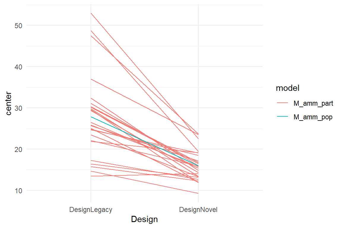
Figure 6.7: Spaghetti plot combining the results of a population-level with a participant-level model
The convenience of (true) multi-level models is that both (or more) levels are specified and estimated as one model. For the multi-level models that follow, we will use a specialized engine, brm() (generalized multi-level regression) that estimates both levels simultaneously and produce multi-level coefficients. The multi-level CGM we desire is written like this:
M_mlcgm <-
  D_pumps %>%
  brm(ToT ~ 1 + Design + (1 + Design | Part), data = .)
In the formula of this multi-level CGM the predictor term (1 + Design) is just copied. The first instance is the usual population-level averages, but the second is on participant-level. The | operator in probability theory means “conditional upon” and here this can be read as effect of Design conditional on participant.
For linear models we have been using the coef() command to extract all coefficients. Here it would extract all coefficients on both levels. With multi-level models, two specialized command exist to separate the levels: we can extract population-level effects using the fixef() command for fixed effects (Table 6.11). All lower level effects can be accessed with the ranef command, which stands for random effects. Random effects are differences towards the population-level. This is why random effects are always centered at zero. In the following histogram, the distribution of the DesignNovel random effects are shown. This is how much users deviate from the average effect in the population (Figure 6.8))
fixef(M_mlcgm)| fixef | center | lower | upper |
|---|---|---|---|
| Intercept | 27.6 | 23.7 | 31.54 |
| DesignNovel | -11.7 | -15.3 | -8.05 |
ranef(M_mlcgm) %>%
  rename(Part = re_entity, `deviation` = center) %>%
  ggplot(aes(x = deviation)) +
  facet_grid(~fixef) +
  geom_histogram()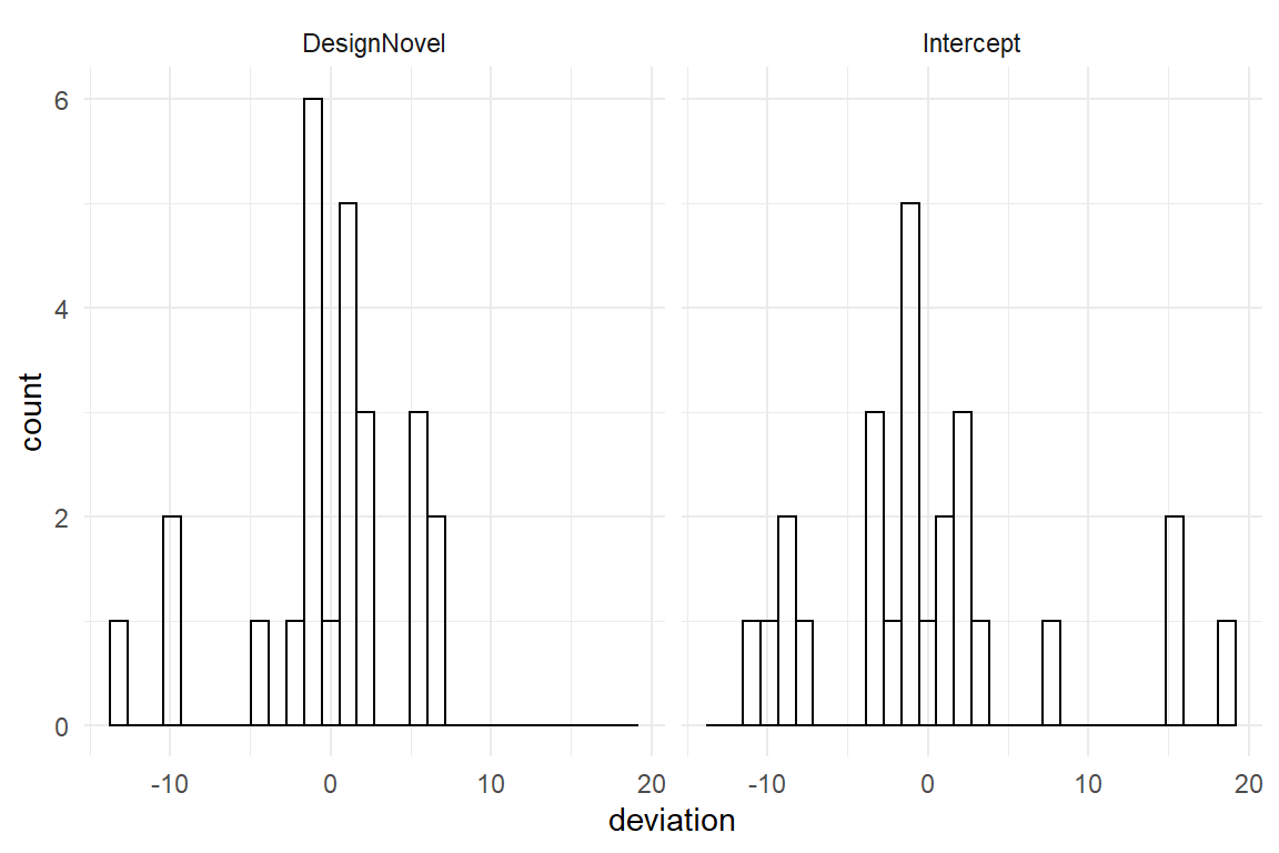
Figure 6.8: Participant-level random effects in a CGM
The distribution of random effects should resemble a Gaussian distribution. It is usually hard to tell with such small sample sizes, but it seems that the Intercept effects have a left skew. As we will see in chapter 7, this problem is not surprising and can be resolved. The distributions are also centered at zero, which is not a coincidence, but the way random effects are designed: deviations from the population mean. That opens up two interesting perspectives: first, random effects look a lot like residuals 4.1.2, and like those we can summarize a random effects vector by its standard deviation, using the grpef command from package Bayr (Table 6.12).
grpef(M_mlcgm)| fixef | center | lower | upper |
|---|---|---|---|
| Intercept | 8.71 | 6.03 | 12.47 |
| DesignNovel | 6.02 | 2.98 | 9.82 |
Most design research is located on the population level. We want to know how a design works, broadly. Sometimes, stratified samples are used to look for conditional effects in (still broad) subgroups. Reporting individual differences makes little sense in such situations. The standard deviation summarizes individual differences and can be interpreted the degree of diversity. The command bayr::fixef_ml is implementing this by simply attaching the standard deviation center estimates to the respective population-level effect (Table 6.13). As coefficients and standard deviations are on the same scale, they can be compared. Roughly speaking, a two-thirds of the population is contained in an interval twice as large as the SD.
fixef_ml(M_mlcgm)| fixef | center | lower | upper | SD_Part |
|---|---|---|---|---|
| Intercept | 27.6 | 23.7 | 31.54 | 8.71 |
| DesignNovel | -11.7 | -15.3 | -8.05 | 6.02 |
That having said, I believe that more researchers should watch their participant levels more closely. Later, we will look at two specific situations: psychometric models have the purpose of measuring individuals 6.8 and those who propose universal theories (i.e., about people per se) must also show that their predictions hold for each and everyone 6.4.
6.4 Testing universality of theories
Often, the applied researcher is primarily interested in a population-level effect, as this shows the average expected benefit. If you run a webshop, your returns are exchangeable. One customer lost can be compensated by gaining a new one. In such cases, it suffices to report the random effects standard deviation. If user performance varies strongly, this can readily be seen in this one number.
In at least two research situations, going for the average is just not enough: when testing hazardous equipment and when testing theories. In safety critical research, such as a medical infusion pump, the rules are different than for a webshop. The rules are non-compensatory, as the benefit of extreme high performance on one patient cannot compensate the costs associated with a single fatal error on another patient. For this asymmetry, the design of such a system must enforce a robust performance, with no catastrophes. The multi-level analysis of the infusion pumps in 6.3 is an example. It demonstrated that practically all nurses will have a benefit from the novel design.
The other area where on-average is not enough, is theory-driven experimental research. Fundamental behavioural researchers are routinely putting together theories on The Human Mind and try to challenge these theories. For example the Uncanny Valley effect 5.5: one social psychologist’s theory could be that the Uncanny Valley effect is caused by religious belief, whereas a cognitive psychologist could suggest that the effect is caused by a category confusion on a fundamental processing level (seeing faces). Both theories make universal statements, about all human beings. Universal statements can never be proven, but can only be hardened. However, once a counter-example is found, the theory needs to be abandonded. If there is one participant who is provenly non-religious, but falls into the Uncanny Valley, our social psychologist would be proven wrong. If there is a single participant in the world, who is robvust against the Uncanny Valley, the cognitive psychologist was wrong.
Obviously, this counter-evidence can only be found on participant level. In some way, the situation is analog to robustness. The logic of universal statements is that they are false if there is one participant who breaks the pattern, and there is no compensation possible. Unfortunately, the majority of fundamental behavioural researchers, have ignored this simple logic and still report population-level estimates when testing universal theories. In my opinion, all these studies should not be trusted, before a multi-level analysis shows that the pattern exists on participant level.
In 5.5, the Uncanny Valley effect has been demonstrated on population level. This is good enough, if we just want to confirm the Uncanny Valley effect as an observation, something that frequently happens, but not necessarily for everyone. The sample in our study consisted of mainly students and their closer social network. It is almost certain, that many of the tested persons were religious and others were atheists. If the religious-attitude theory is correct, we would expect to see the Uncanny Valley in several participants, but not in all. If the category confusion theory is correct, we would expect all participants to fall into the valley. The following model performs the polynomial analysis as before 5.5, but multi-level:
attach(Uncanny)M_poly_3_ml <-
RK_1 %>%
brm(response ~ 1 + huMech1 + huMech2 + huMech3 +
(1 + huMech1 + huMech2 + huMech3 | Part),
data = ., iter = 2500
)
P_poly_3_ml <- posterior(M_poly_3_ml)
PP_poly_3_ml <- post_pred(M_poly_3_ml, thin = 5)One method for testing universality is to extract the fitted responses (predict) and perform a visual examination: can we see a valley for every participant?
T_pred <-
  RK_1 %>%
  mutate(M_poly_3_ml = predict(PP_poly_3_ml)$center)

T_pred %>%
  ggplot(aes(x = huMech, y = M_poly_3_ml, group = Part)) +
  geom_smooth(se = F, size = .5) +
  labs(x = "human likeness", y = "fitted emotional response")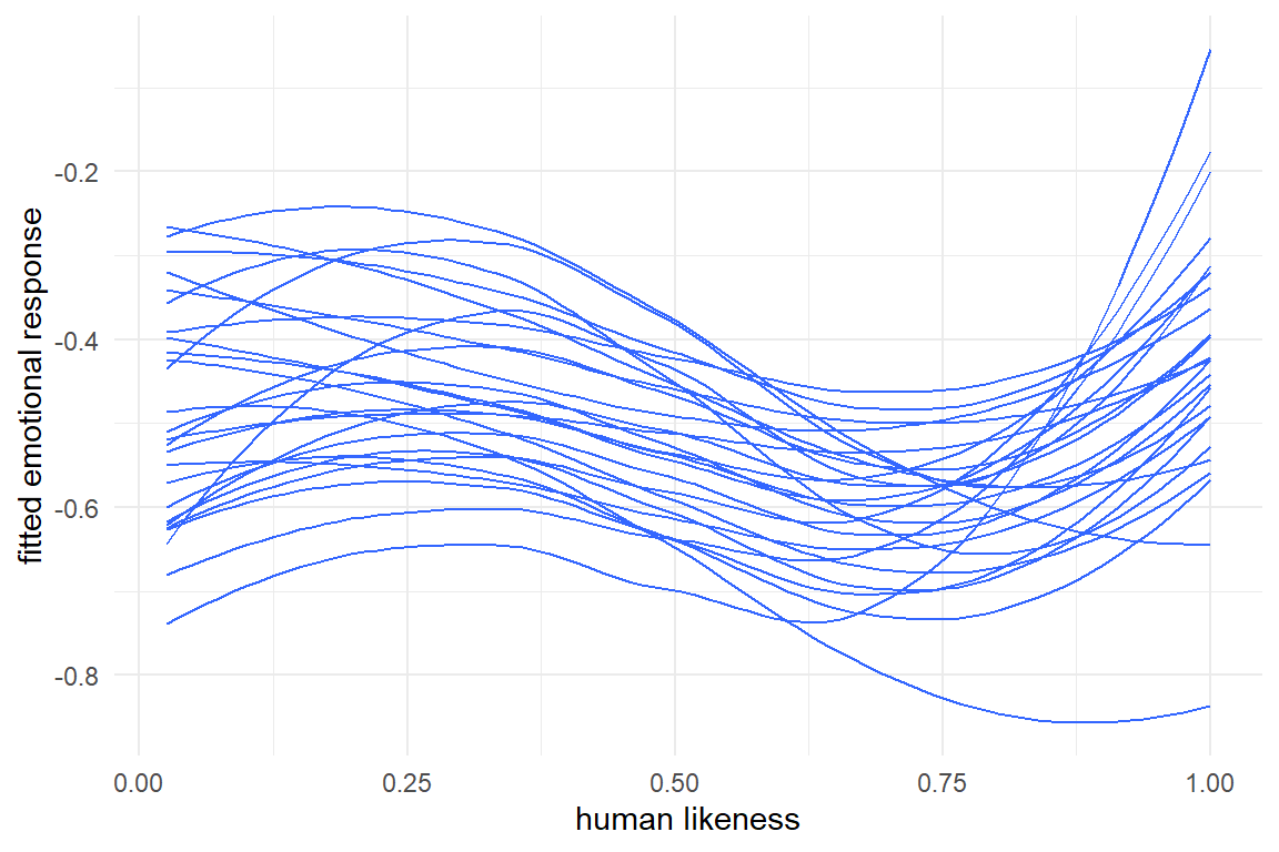
Figure 6.9: Participant-level associations between human likeness and
This spaghetti plot broadly confirms, that all participants experience the Uncanny Valley. For a more detailed analysis, a facetted plot would be better suited, allowing to inspect the curves case-by-case.
We proceed directly to a more formal method of testing universality: In 5.5.1 we have seen how the posterior distributions of shoulder and trough can be first derived and then used to give a more definitive answer on the shape of the polynomial. It was argued that the unique pattern of the Uncanny Valley is to have a shoulder left of a trough. These two properties can be checked by identifying the stationary points. The proportion of MCMC iterations that fulfill these properties can is evidence that the effect exists.
For testing universality of the effect, we just have to run the same analysis on participant-level. Since the participant-level effects are deviations from the population-level effect, we first have to add the population level effect to the random effects (using the Bayr command re_scores), which creates absolute polynomial coefficients. The two commands trough and shoulder from package Uncanny require a matrix of coefficients, which is done by spreading out the posterior distribution table. Then all the characteristics of the polynomial are checked, that define the Uncanny Valley phenomenon:
- a trough
- a shoulder
- the shoulder is left of the trough
# devtools::install_github("schmettow/uncanny")

library(uncanny)

P_univ_uncanny <-
  P_poly_3_ml %>%
  re_scores() %>%
  select(iter, Part = re_entity, fixef, value) %>%
  tidyr::spread(key = "fixef", value = "value") %>%
  select(iter, Part, huMech0 = Intercept, huMech1:huMech3) %>%
  mutate(
    trough = trough(select(., huMech0:huMech3)),
    shoulder = shoulder(select(., huMech0:huMech3)),
    has_trough = !is.na(trough),
    has_shoulder = !is.na(shoulder),
    shoulder_left = trough > shoulder,
    is_uncanny = has_trough & has_shoulder & shoulder_left
  )
To produce Figure 6.10, the probability that the participant experienced the Uncanny Valley is calculated as the proportion (mean) of MCMC samples that meet the criteria.
P_univ_uncanny %>%
  group_by(Part) %>%
  summarize(prob_uncanny = mean(is_uncanny)) %>%
  mutate(label = str_c(100 * round(prob_uncanny, 4), "%")) %>%
  ggplot(aes(x = Part, y = prob_uncanny)) +
  geom_col() +
  geom_label(aes(label = label)) +
  theme(axis.text.x = element_text(angle = 45))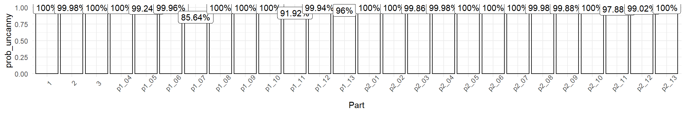
Figure 6.10: Participant-level certainty that the Uncanny Valley phenomenon happened
Figure 6.10 gives strong support to the universality of the Uncanny Valley. What may raise suspicion is rather that for most participants the probability is 100%. If this is all based on a random walk, we should at least see a few deviations, shouldn’t we. The reason for that is that MCMC samples approximate the posterior distribution by frequency. As their is a limited number of samples (here: 4000), the resolution is limited. If we increase the number of iterations enough, we would eventually see few “deviant” samples appear and measure the tiny chance that a participant does not fall for the Uncanny Valley.
This is great news for all scientists who believe that the Uncanny Valley effect is an innate cognitive phenomenon (rather than cultural). The same technique can also be used for the identification of deviant participants, those few that are totally against the trend. We briefly re-visit case Sleepstudy, for which we have estimated a multi-level linear regression model to render individual increase of reaction time as result of sleep deprivation (6.2). By visual inspection, we identified a single deviant participant who showed an improvement over time, rather than a decline. However, the fitted lines a based on point estimates, only (the median of the posterior). Using the same technique as above, we can calculate the participant-level probabilities for the slope being positive, as expected.
attach(Sleepstudy)P_scores <-
posterior(M_slpsty_1) %>%
re_scores() %>%
mutate(Part = re_entity)
P_scores %>%
filter(fixef == "days") %>%
group_by(Part) %>%
summarize(prob_positive = mean(value >= 0)) %>%
mutate(label = str_c(100 * round(prob_positive, 4), "%")) %>%
ggplot(aes(x = Part, y = prob_positive)) +
geom_col() +
geom_label(aes(label = label), vjust = 1) +
theme(axis.text.x = element_text(angle = 45))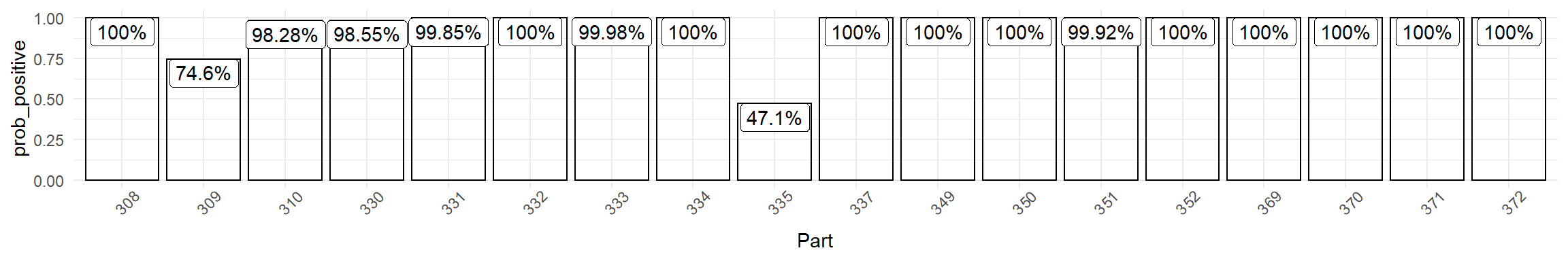
Figure 6.11: Participant-level certainty that the Uncanny Valley phenomenon happened
All, but participants 309 and 335, almost certainly have positive slopes. Participant 335 we had identified earlier by visual inspection. Now, that we account for the full posterior distribution, it seems less suspicious. There is almost a 50% chance that the participant is suffering from sleep deprivation, too. Figure 6.12 is an attempt at illustrating the uncertainty. It shows all the possible slopes the MCMC random walk has explored from (unsuspicious) participant 308 and participant 335. While the latter has a distinctly different distribution, there is no compelling reason to get too excited and call 335 a true counter-example from the rule that sleep deprivation reduces cognitive performance.
P_scores %>%
  filter(Part %in% c(308, 335), fixef == "days") %>%
  ggplot() +
  xlim(0.05, 1) +
  ylim(-10, 25) +
  geom_abline(aes(intercept = 0, slope = value),
    alpha = .01
  ) +
  facet_grid(. ~ Part)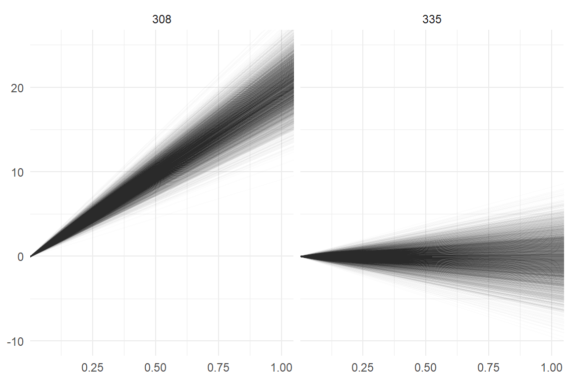
Figure 6.12: Visualizing the uncertainty in Days for two pareticipants
In turn, the method of posterior-based test statistics can also be used for analysis of existence. In the Sleepstudy case a hypothetical question of existence would be that there exist persons who are completely insensitive to sleep deprivation. Why not? Recently, I saw a documentary about a guy who could touch charged electric wires, because due to a rare genetic deviation, his skin had no sweat glands. Whereas universal statements can only be falsified by a counter-example, statements of existence can be proven by just a single case. For example, in the 1980 dyslexia became more widely recognized as a defined condition. Many parents finally got an explanation for the problems their kids experienced in school. Many teachers complained that many parents would just seek cheap excuses for their lesser gifted offsprings. And some people argued that dyslexia does not exist and that the disability to read is just a manifestation of lower intelligence. According to the logic of existence, a single person with a well functioning intellect, but hampered reading suffices to proof the existence of dyslexia. These people have been found in the meantime.
6.5 Non-human populations and cross-overs
With multi-level models design researchers can examine how a design affects the population of users as a whole, as well as on individual level. If there is little variation between users, it can be concluded that the effect is uniform in the population of users. In this section we will generalize the term population and extend the application of multi-level modeling to other types of research entities, such as designs, questionnaire items and tasks.
Many studies in, what one could call fundamental design research seek to uncover general laws of design that may guide future system development. Fundamental design research is not concerned with choosing between individual designs, whether they are good enough or not, but with separating the population of possible designs into good ones and bad ones by universal statements, such as “For informational websites, broad navigation structures are better than deep ones.” Note how this statement speaks of designs (not users) in an unspecified plural. It is framed as a universal law for the population of designs.
Comparative evaluation studies, such as the IPump case, are not adequate to answer such questions, simply because you cannot generalize to the population from a sample of two. This is only possible under strict constraints, namely that the two designs under investigation only differ in one design property. For example two versions of a website present the same web content in a deep versus a wide hierarchy, but layout, functionality are held constant. And even then, we should be very careful with conclusions, because there can be interaction effects. For example, the rules could be different for a website used by expert users.
If the research question is universal, i.e. aiming at general conclusions on all designs (of a class), it is inevitable to see designs as a population from which we collect a sample. The term population suggests a larger set of entities, and in fact many application domains have an abundance of existing designs and a universe of possible designs. Just to name a few: there exist dozens of note taking apps for mobile devices and hundreds of different jump’n run games. Several classes of websites count in the ten thousands, such as webshops, municipal websites or intranets.
We can define classes of objects in any way we want, but the term population, has a stronger meaning than just a collection. A population contains individuals of the same kind and these individuals vary, but only to some extent. At the same time, it is implied that we can identify some sort of typical value for a population, such that most individuals are clumped around this typical value. Essentially, if it looks similar to one of the basic statistical distributions 3.5.2, we can call it a population.
To illustrate that not every class is a population, take vehicles. Vehicles are a class of objects that transport people or goods. This broad definition covers many types of vehicles, including bicycles, rikshas, cars, buses, trucks and container vessels. If the attribut under question is the weight, we will see a distribution spreading from a 10 kilograms up to 100 tons (without freight). That is a a scale of 1:10.000 and the distribution would spread out like butter on a warm toast. Formally, we can calculate the average weight of a all vehicles, but that would in no way represent a typical value.
In design research the most compelling populations are users and designs. Besides that research objects exist that we can also call members of a population, such as tasks, situations and questionnaire items.
Tasks: Modern informational websites contain thousands of information pieces and finding every one of those can be considered a task. At the same time, it is impossible to cover them all in one study, such that sampling a few is inevitable. We will never be able to tell the performance of every task, but using random effects it is possible to estimate the variance of tasks. Is that valuable information? Probably it is in many cases, as we would not easily accept a design that prioritizes on a few items at the expense of many others, which are extremely hard to find.
Situations: With the emerge of the web, practically everyone started using computers to find information. With the more recent breakthrough in mobile computing, everyone is doing everything using a computer in almost every situation. People chat, listen to music and play games during meals, classes and while watching television. They let themselves being lulled into sleep, which is tracked and interrupted by smart alarms. Smartphones are being used on trains, while driving cars and bikes, however dangerous that might be, and not even the most private situations are spared. If you want to evaluate the usability of any mobile messaging, navigation and e-commerce app, you should test it in all these situations. A study to examine performance across situations needs a sample from a population of situations.
Questionnaire items: Most design researchers cannot refrain from using questionnaires to evaluate certain elucive aspects of their designs. A well constructed rating scale consists of a set of items that trigger similar responses. At the same time, it is desireable that items are unsimilar to a degree, as that establishes good discrimination across a wide range. In ability tests, for example to assess people’s intelligence or math skills, test items are constructed to vary in difficulty. The more ability a person has, the more likely will a very difficult item be solved correctly. In design research, rating scales cover concepts such as perceived mental workload, perceived usability, beauty or trustworthiness. Items of such scales differ in how extreme the proposition is, like the following three items that could belong to a scale for aesthetic perception:
- The design is not particularly ugly.
- The design is pretty.
- The design is a piece of art.
For any design it is rather difficult to get a positive response on item 3, whereas item 1 is a small hurdle. So, if one thinks of all possible propositions about beauty, any scale is composed of a sample from the population of beauty propositions.
If we look beyond design research, an abundance of non-human populations can be found in other research disciplines, such as:
- products in consumer research
- phonemes in psycholinguistics
- test items in psychometrics
- pictures of faces in face recognition research
- patches of land in agricultural studies
- households in socio-economic studies
In all these cases it is useful (if not inevitable) to ask multi-level questions not just on the human population, but on the encounter of multiple populations. In research on a single or few designs, such as in A/B testing, designs are usually thought of (and modeled) as common fixed-effects factors. However, when the research question is more fundamental, such that it regards a whole class of designs, it is more useful to think of designs as a population and draw a sample. In the next section we will see an example, where a sample of users encounters a sample of designs and tasks.
In experimental design research, the research question often regards a whole class of designs and it is almost inevitableto view designs as a population. As we usually want to generalize across users, that is another sample. A basic experimental setup would be to have every user rate (or do a task) on every design, which is called a complete (experimental) design, but I prefer to think of it as a complete encounter.
Every measure is an encounter of one participant and one design. But, if a multi-item rating scale is used, measures are an encounter between three populations. Every measure combines the impact from three members from these populations. With a single measure, the impact factors are inseparable. But if we have repeated measures on all populations, we can apply a cross-classified multi-level model (CRMM). An intercept-only CRMM just adds intercept random effects for every population.
In the following case Egan, the question is a comparison of diversity across populations. Three decades ago, (Egan 1988) published one of the first papers on individual differences in computer systems design and made the following claim:
‘differences among people usually account for much more variability in performance than differences in system designs’
What is interesting about this research question is that it does not speak about effects, but about variability of effects and seeks to compare variability of two totally different populations. In the following we will see how this claim can be tested by measuring multiple encounters between populations
Egan’s claim has been cited in many papers that regarded individual differences and we were wondering how it would turn out in the third millennium, with the probably most abundant of all application domains: informational websites. For the convenience, we chose the user population of student users, with ten university websites as our design sample. Furthermore, ten representative tasks on such websites were selected, which is another population. During the experiment, all 41 participants completed 10 information search items such as:
On website [utwente.nl] find the [program schedule Biology].
attach(Egan)Note that ToT is log-transformed for compliance with the assumptions of Linear Models. Generally, the advice is to use a Generalized Linear Model instead 7.3.2. Egan’s claim is a two-way encounter to which we added the tasks, which makes it three-way. However, our data seemed to require a fourth random effect, which essentially is a conditional effect between tasks and websites, which we call an item. Figure 6.13 shows a grid of histogram with the marginal distributions of human and non-human populations. The individual plots were created using the following code template:
D_egan %>%
  group_by(Part) %>%
  summarize(avg_logToT = mean(logToT)) %>%
  ggplot(aes(x = avg_logToT)) +
  geom_histogram() +
  labs(title = "participant-level average log-times") +
  xlim(1.5, 6.5)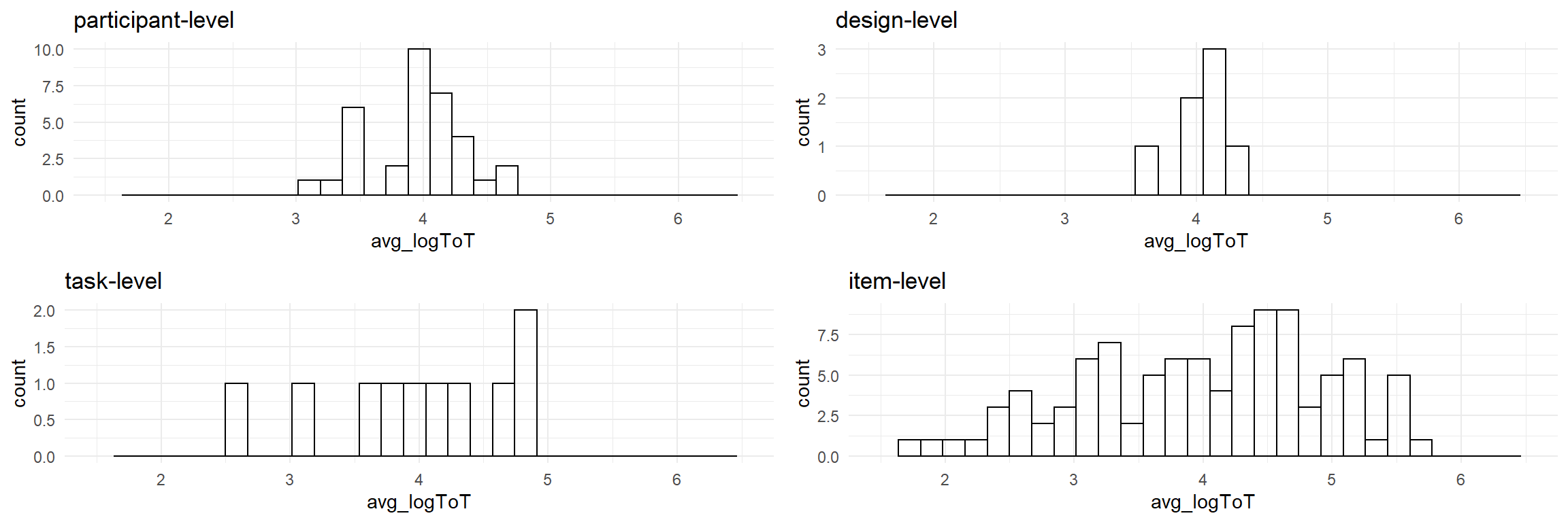
Figure 6.13: Distribution of human and non-human populations in the Egan experiment (scale log(ToT))
There seems to be substantial variation between participants, tasks and items, but very little variation in designs. We build a GMM for the encounter of the four populations.
M_1 <-
  brm(logToT ~ 1 +
    (1 | Part) + (1 | Design) + (1 | Task) + (1 | Design:Task),
  data = D_egan
  )

P_1 <- posterior(M_1)
A Bayesian multi-level model estimates the standard deviation alongside with coefficients, such that we can compare magnitude and certainty of variability. In addition, we include the standard error as an observation-level effect (Obs) for comparison (Figure 6.14).
library(mascutils) # reorder-levels

P_1 %>%
  filter(type == "grpef" | type == "disp") %>%
  mutate(
    re_factor = if_else(type == "disp",
      "Obs", re_factor
    ),
    re_factor = reorder_levels(
      re_factor,
      c(4, 2, 5, 3, 1)
    )
  ) %>%
  ggplot(aes(x = value)) +
  geom_density() +
  labs(x = "random effect standard deviation") +
  facet_grid(re_factor ~ .)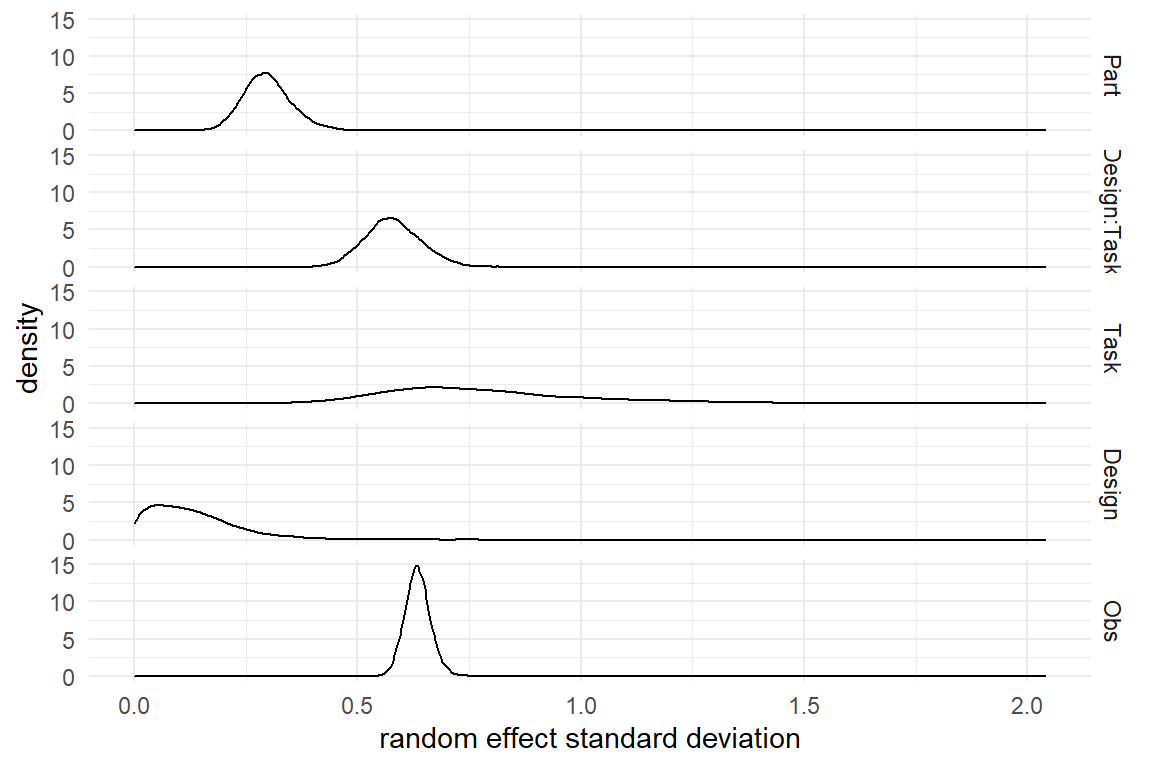
Figure 6.14: Density plot of random effects standard deviations.
The outcomes of our study are indecisive regarding Egan’s claim. Variance of participants is stronger than variance of designs, but the posterior distributions overlap a good deal. Both factors also produce much less variability in measures than does the remaining noise. Tasks seem to have the overall strongest effect, but this comes with huge uncertainty. The strongest variability is found in the sample of items (Design x Task), which is an interesting observation. How easy a task is, largely depends on the website where it is carried out. That makes sense, as all pieces of information somehow compete for space. For example, one university website could present the library on the homepage, whereas another websites hides it deep in its navigation structure.
A secondary observation on the posterior plot is that some effects are rather certain, such as Obs and Design:Task, whereas others are extremely uncertain, especially Task. There is a partial explanation for this: the variation is estimated from the “heads” in thehuman or non-human population. It therefore strongly depends on respective sample size. Design and Task have a meager \(N = 10\), which is why the estimate are so uncertain. With \(N = 41\) the participant level estimate has more data and reaches better certainty, same for the pairs (\(N = 100\)). The observations level can employ to all 410 observations, resulting in a highly certain estimate.
Still, Egan’s claim is out in the world and requires an answer. To reduce the quantitative findings to a Yes/No variable, we use the same technique as in 5.5.1 and 6.4. What is the probability, that Egan is right? We create a Boolean variable and summarize the proportion of MCMC draws, where \(\sigma_ \textrm{Part} > \sigma_ \textrm{Design}\) holds.
P_1 %>%
  filter(type == "grpef", re_factor %in% c("Part", "Design")) %>%
  select(chain, iter, re_factor, value) %>%
  spread(re_factor, value) %>%
summarize(prob_Egan_is_right = mean(Part > Design)) | prob_Egan_is_right |
|---|
| 0.928 |
Such a chance can count as good evidence in favor of Egan’s claim, although it certainly does not match the “much more” in the original quote. However, if we take the strong and certain Item effect (Design x Task) into account, the claim could even be reversed. Apparently, the difficulty of a task depends on the design, that means, it depends on where this particular designer has placed an item in the navigation structure. These are clearly design choices and if we see it this way, evidence for Egan’s claim is practically zero (.0005, Table 6.15).
P_1 %>%
  filter(type == "grpef", re_factor %in% c("Part", "Design", "Design:Task")) %>%
  select(chain, iter, re_factor, value) %>%
  spread(re_factor, value) %>%
  mutate(Egan_is_right = Part > Design & Part > `Design:Task`) %>%
summarize(prob_Egan_is_right = mean(Egan_is_right)) | prob_Egan_is_right |
|---|
| 5e-04 |
In this section we have seen that measures in design research happen in encounters between users, designs and several other non-human populations. Cross-classified random effects models capture these structures. When testing Egan’s claim, we saw how an exotic hypothesis such as the difference in variance, can be answered probabilistically, because with Bayesian models, we get posterior distributions for all parameters in a model, not just coefficients.
6.6 Nested random effects
In some research designs, we are dealing with populations that have a hierarchical structure, where every member is itself composed of another population of entities. A classic example is from educational research: schools are a non-human population, underneath which we find a couple of other populations, classes and students. Like cross-classified models, nested models consist of multiple levels. The difference is that if one knows the lowest (or: a lower) level of an observation, the next higher level is unambiguous, like:
- every class is in exactly one school
- every student is in exactly one school (or class)
Nested random effects (NRE) represent nested sampling schemes. As we have seen above, cross-classified models play an important role in design research, due to the user/task/design encounter. NREs are more common in research disciplines where organisation structures or geography plays a role, such as education science (think of the international school comparison studies PISA and TIMMS), organisational psychology or political science.
One examples of a nested sampling structure in design research is the CUE8 study, which is the eighth instance of Comparative Usability Evaluation (CUE) studies by Rolf Molich (Molich et al. 2010). Different to what the name might suggest, not designs are under investigation in CUE, but usability professionals. The over-arching question in the CUE series is the performance and reliability of usability professionals when evaluating designs. Earlier studies sometimes came to devastating results regarding consistency across professional groups when it comes to identifying and reporting usability problems. The CUE8 study lowered the bar, by asking if professionals can at least measure time in a comparable way.
The CUE8 study measured time-on-task in usability tests, which had been conducted by 14 different teams. The original research question was: How reliable are time-on-task measures across teams? All teams used the same website (a car rental company) and the same set of tasks. All teams did moderated or remote testing (or both) and recruited their own sample of participants (Table 6.16)).
attach(CUE8)

D_cue8| Obs | Team | Part | Condition | SUS | Task | ToT | logToT |
|---|---|---|---|---|---|---|---|
| 267 | D3 | 54 | remote | 2 | 135 | 4.91 | |
| 527 | G3 | 106 | moderated | 2 | 89 | 4.49 | |
| 689 | H3 | 138 | remote | 33.0 | 4 | 28 | 3.33 |
| 899 | J3 | 180 | remote | 4 | 367 | 5.91 | |
| 993 | K3 | 199 | moderated | 72.5 | 3 | 61 | 4.11 |
| 1318 | L3 | 264 | remote | 73.0 | 3 | 69 | 4.23 |
| 1879 | L3 | 376 | remote | 98.0 | 4 | 105 | 4.65 |
| 2327 | M3 | 466 | remote | 77.5 | 2 | 213 | 5.36 |
An analysis can performed on three levels: the population level would tell us the average performance on this website. That could be interesting for the company running it. Below that are the teams and their variation is what the original research question is about. Participants make the third level for a nested multi-level model. It is nested, because every participant is assigned to exactly one team. If that weren’t the case, say there is one sample of participants shared by the teams, that would be cross-classification.
As the original research question is on the consistency across teams, we can readily take the random effect variance as a measure for the opposite: when variance is high, consistency is low. But, how low is low? It is difficult to come up with an absolute standard for inter-team reliability. Because we also have the participant-level, we can resort to a relative standard: how does the variation between teams compare to variation between individual participants?
Under this perspective, we examine the data. This time, we have real time-on-task data and as so often, it is highly skewed. Again, we use the trick of logarithmic transformation to obtain a more symmetric distribution of residuals. The downside is that the outcome variable may not be zero. For time-on-task data this is not an issue. Before proceeding to the model, we explore the original variable ToT on the two levels (Participant and Team). In the following code the mean ToT is computed for the two levels of analysis, participants and teams and shown in ascending order (Figure 6.15).
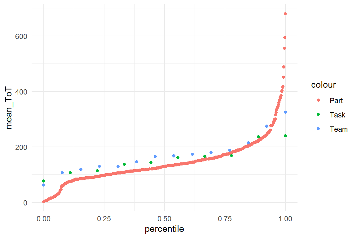
Figure 6.15: Distribution of mean scores on three levels
It seems there is ample variation in ToT for participants, with mean ToT ranging from below 100 to almost 500 seconds. There also is considerable variation on team level, but the overall range seems to be a little smaller. Note, however, that the participant level contains all the variation that is due to teams. A model with nested random effects can separate the sources of variation. When two (or more) levels are nested, a special syntax applies for specifying nested random effects. 1|Team/Part.
M_1 <-
  D_cue8 %>%
  brm(logToT ~ Condition + (1 | Team / Part),
    data = .
  )

P_1 <- posterior(M_1)
Note that the model contains another feature of the CUE8 study the effect of the testing condition, moderated or remote. Why does this not have a participant-level effect. As participants are either moderated or remote, we simply don’t get any data, on how the same participant behaved in the other condition.
P_1| model | parameter | type | fixef | re_factor | count |
|---|---|---|---|---|---|
| M_1 | ranef | Intercept | Team | 14 | |
| M_1 | ranef | Intercept | Team:Part | 523 | |
| M_1 | b_Conditionmoderated | fixef | Conditionmoderated | 1 | |
| M_1 | b_Intercept | fixef | Intercept | 1 | |
| M_1 | sigma | disp | |||
| M_1 | sd_Team:Part__Intercept | grpef | Intercept | ||
| M_1 | sd_Team__Intercept | grpef | Intercept |
The posterior object reveals two random factors, one for teams and one for participants. The interpretation is in no way different than cross-classified random effects. In both cases, the absolute group mean for a certain participant is obtained by adding up all two coefficients.
The syntax really is just a safe way to deal with nested samples, where participant identifiers could be re-used. If participant identifiers were unique (Table 6.18), a cross-classified model with the formula logToT ~ Condition + (1|Part) + (1|Team) would produce the exact same results.
D_cue8_x <-
  D_cue8 %>%
  unite(Part, Team:Part, remove = F) %>%
  as_tbl_obs()

D_cue8_x| Obs | Part | Team | Condition | SUS | Task | ToT | logToT |
|---|---|---|---|---|---|---|---|
| 188 | C3_38 | C3 | moderated | 3 | 67 | 4.21 | |
| 842 | J3_169 | J3 | remote | 2 | 147 | 4.99 | |
| 958 | K3_192 | K3 | moderated | 97.5 | 3 | 80 | 4.38 |
| 1127 | L3_226 | L3 | remote | 100.0 | 2 | 193 | 5.26 |
| 1557 | L3_312 | L3 | remote | 100.0 | 2 | 247 | 5.51 |
| 1901 | L3_381 | L3 | remote | 80.0 | 1 | 133 | 4.89 |
| 2314 | M3_463 | M3 | remote | 70.0 | 4 | 224 | 5.41 |
| 2386 | M3_478 | M3 | remote | 92.5 | 1 | 104 | 4.64 |
Let’s take a closer look at the results regarding consistency of ToT measures across teams (Table 6.19). We would always expect participants to show variation, but if team averages show strong variation, then we can suspect that there are biases. It turns out that the variation by team is by a factor of 1.5 larger than individual differences. And it is on par with the measurement error (sigma).
P_1 %>%
  filter(type %in% c("fixef", "grpef")) %>%
clu()| parameter | fixef | re_factor | center | lower | upper |
|---|---|---|---|---|---|
| b_Intercept | Intercept | 4.629 | 4.062 | 5.19 | |
| b_Conditionmoderated | Conditionmoderated | 0.326 | -0.393 | 1.12 | |
| sd_Team__Intercept | Intercept | Team | 0.619 | 0.417 | 1.01 |
| sd_Team:Part__Intercept | Intercept | Team:Part | 0.428 | 0.390 | 0.47 |
It is not surprising to see the test users vary greatly in performance. What is concerning is that the discordance between professional teams. Note that this is the net variance after controlling for the condition, remote or moderated. Surprisingly, evidence for just that difference rather low and highly uncertain (\(0.33 [-0.39, 1.12]_{CI95}\)).
In this section we introduced a new perspective on multi-level models. Here, the question was to quantify and compare samples (rather than conditions) as sources of variation. With multi-level models, we can separate sources of variation. This builds on how random effects are constructed, as factor levels drawn from a Gaussian distribution. In the following section, we will delve deeper into the matter of random effects.
6.7 What are random effects? On pooling and shrinkage
At least half a dozen of definitions exist for the term random effect. This is so confusing that some authors refrain to use the term altogether. In addition, the very terms random effect and random factor are highly misleading, as there is nothing more or less random in a random factors as compared to fixed factors. Here, the definition of a random effects is conceptually based on the idea of a population, and implemented as a factor, where levels are assumed to follow a Gaussian distribution.
A Gaussian distribution extends in both directions infinitely, but the extreme tails are becoming very thin. The low assigned probability of extreme events acts on the estimate, by correcting extreme estimates towards the mean, which is called shrinkage.
When a data set contains a factor that we may wish to add to the model, the question is: fixed effect or random effect? In 6.5, I have introduced the heuristic of populations. If one can conceive tasks, designs, or whatever set of items as a population, there is clumping to some degree, but also variation. The more clumping there is, the better is the guess for unobserved members by observing some members.
Obviously, we would never speak of a population, when the objects of interest are from different classes. Entities gathering on super market parking lots, like persons, cars, baskets and and dropped brochures, we would never see as a population. People, we would generally see as a population, as long as what we want to observe is somewhat comparable between members. When the question is, how fast persons can do a 2000 meter run at the Olympic games, we would certainly want one population per discipline (swimming, running, etc). Why is that so? It is because we expect members of a population to have some similarity, with the consequence that, if you already have observed some members of the population, this tells you something about any unobserved members.
Reconsider the Bayesian principle of prior knowledge by an experiment of thought: Consider, a UX expert with experience in e-commerce is asked to estimate how long it takes users to do the checkout, but without showing the expert the actual system. The expert will probably hesitate briefly, and then come up with an estimate of, let’s say, 45 seconds. Without any data, the expert made some reasonable assumptions, e.g. that a disciplined design process has been followed, and then relies on experience. The experts personal experience has formed prior to the study by observing many other cases. Now, we confront the expert with an even more bizzare situation: guess the time-on-task for an unknown task with an unseen system of unknown type! The expert will probably refuse to give an answer, arguing that some systems have tasks in the second range (e.g. starting a car), whereas other processes easily run for hours or days (e.g. writing a report). This is a good point and the expert is provided, not with knoeledge of the system, but with average ToT of four other tasks within the same system:
\(ToT_{1-4} = {23, 45, 66, 54}\)
Now, the expert is confident that ToT be around 50 seconds and that is probably a good guess. What has happened is that prior belief about the unkown task parameter has been formed not externally, but by data as it arrived. The likely value of one unit has been learned from the other units and this appears pretty reasonable. The same principle applies when visually identifying outliers in a boxplot or scatterplot. First, the mind of the observer forms a gestalt that covers the salient features of data, for example: almost all points are located in the range 100 - 500. Once this pattern has formed, deviant points stand out.
However, the salience of the gestalt may vary. Consider a situation where ToT has been measured by the same procedure, but using five different stop watches. Stop watches are so incredibly accurate that if you know one measure, you basically know them all. What many researchers do with repeated measures data, is take the average. This is the one extreme called total pooling. In the stopwatch case the average of the five measures would be so highly representative, that total pooling is a reasonable thing to do.
In other cases, the levels of a factor are more or less independent, for example tasks in a complex system, where procedure duration ranges from seconds to hours. Guessing the duration of one task from a set of others is highly susceptible and the average duration across tasks is not representative at all. The best choice then is to see tasks as factor levels, that are independent. This extreme of no pooling is exactly represented by fixed effect factors as they have been introduced in 4.
Random effects sit right between these two extremes of no and total pooling and implement partial pooling: the more the group mean is representative for the units of the group, the more it is taken into account. By this we can also see, why a multi-level model must estimate alle levels simultaneously. The best thing about partial pooling is that, unlike real priors, there is not even the need to determine the amount of pooling in advance. The variation of entities has been observed. The stronger the enities vary, the less can be learned from the group level. The variation is precisely the group-level standard deviation of the random effect.
How are random effects implemented to draw on both sources? Obviously, the procedure must be more refined than just adding participant-level dummy variables into the structural part of the model. In the Bayesian framework a remarkably simple trick suffices, and it is even a familiar one. By the concept of prior distributions, we already know a way to restrict the range of an effect based on prior knowledge. For example, intelligence test results have the prior distribution \(IQ ~ \textrm{Gaus}(100, 15)\), just because they have been empirically calibrated this way. In most other cases, we do have rough ideas about the expected magnitude and range in the population, say: healthy human adults will finish a 2000m run in the range of 5-12 minutes.
As prior knowledge is external to the data, it often lacks systematic evidence, with the exception of a meta analyses. This is why we tend to use weak informative priors. Like priors, random effects take into account knowledge external to the entity under question. But, they draw this knowledge from the data, which is more convincing after all. The basic trick to establish the cross-talk between random factor levels, is to simultaneously estimate factor levels and random factor variation. This has several consequences:
All random effects get a more or less subtle trend towards the population mean. As a side effect, the random factor variance is usually smaller than variance between fixed factors, or naive group means. This effect is called shrinkage. When the random factor variation is small, extreme factor levels are pulled stronger towards the population mean, resulting in stronger shrinkage. Or vice versa: When random variation is large, the factor levels stand more on their own.
The random factor variation is an estimate and as such it is certain only to a degree. As we have seen in 6.5, the more levels a random factor comprises, the more precise is the estimate of random factor variation. The strongest shrinkage occurs with few observations per factor levels and highly certain random factor variation.
Previously, I have stressed how important repeated measures design is, as the number of observations per entity plays a role, too. The more observations there are, the less is the group mean overruled by the population mean. Less shrinkage occurs. This is why multi-level models gracefully deal with imbalanced designs. Groups with more observations are just gradually more self-determined. Taking this to the opposite extreme: when a factor level contains no data at all, it will just be replaced by the population mean. This principle offers a very elegant solution to the problem of missing data. If you know nothing about a person, the best guess is the population mean.
Under the perspective of populations as a more or less similar set of entities, these principles seem to make sense. Within this framework, we can even define what fixed effects are:
a fixed effect is a factor where levels are regarded so unsimilar, that the factor-level variance can be practically considered infinite.
The CUE8 study makes a case for seeing shrinkage in action: Teams of researchers were asked to conduct a performance evaluation on a website. Tasks and website were the same, but the teams followed their own routines. Some teams tested a few handful of participants, whereas others tested dozens remotely. Teams, as another non-human population (sic!) differ vastly in the number of observations they collected. We can expect differences in shrinkage.
To see the effect, we compare the team-level group means as fixed factor versus random factor. All teams have enough participants tested to estimate their mean with some certainty. At the same time, the group sizes vary so dramatically that there should be clear differences in adjustment towards the mean. However, in absolute terms, the sample sizes are very large. There is enough data to estimate team-level scores, and the shrinkage effect is barely visible. For the purpose of demonstration, we use a data set that is reduced to one tenth of the original. We estimate two models, a fixed effects model and a random effects model, from which we collect the (absolute) random effect scores.
attach(CUE8)set.seed(42)
D_cue8_1 <-
D_cue8 %>%
sample_frac(.1)M_2 <-
D_cue8_1 %>%
brm(logToT ~ Team - 1, data = .)
M_3 <-
D_cue8_1 %>%
brm(logToT ~ 1 + (1 | Team), data = .)P_fixef <- posterior(M_2, type = "fixef")
P_ranef <- posterior(M_3) %>%
bayr::re_scores()
T_shrinkage <-
D_cue8_1 %>%
group_by(Team) %>%
summarize(N = n()) %>%
mutate(
fixef = fixef(P_fixef)$center,
ranef = ranef(P_ranef)$center,
shrinkage = fixef - ranef
)T_shrinkage %>%
ggplot(aes(x = Team, size = N)) +
geom_point(aes(y = fixef, col = "fixef"), alpha = .5) +
geom_point(aes(y = ranef, col = "ranef"), alpha = .5) +
geom_hline(aes(yintercept = mean(ranef))) +
labs(color = "Effect type")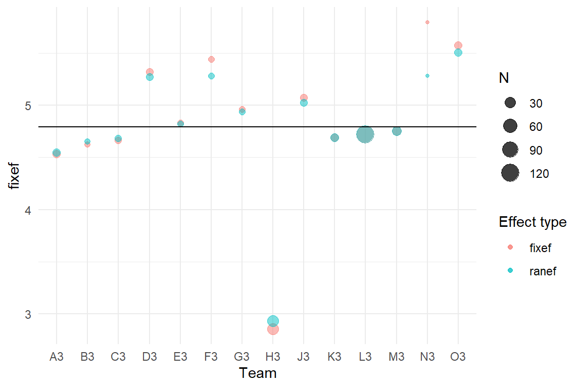
Figure 6.16: Shrinkage shown as disparity of fixed effects and random effects
Figure 6.16 shows how random effects are adjusted towards the grand mean. Groups that are distant (e.g. H, N and O) are more strongly pulled towards the mean. Also, when there is little data in a group, shrinkage is more pronounced (e.g. D, E and G).
In the case of full CUE8 data set, these correction are overall negligible, which is due to the fact that all teams gathered ample data. However, in all situations where there is little or unevenly distributed data, it makes sense to draw more information from the population mean and making inference from random effects is more accurate.
In conclusion, random effects are factors with the additional assumption of Gaussian distribution. When a multi-level model is estimated, the population level effect, the random effects levels and the variance of their distributions are estimated simultaneously. This creates two particular advantages of multi-level models with random effects:
- In unbalanced research designs (with unequal number of observations per subject) small groups are corrected towards the population mean.
- Strong outliers are corrected towards the population mean.
Classical techniques for repeated measures often require additional tweaks to work well with unbalanced designs and outliers. Multi-level models with random effects handle those situations gracefully.
6.8 Psychometrics and design-o-metric models
Random effects apply to all factors, where the levels can be thought of as members of a population (6.5). Looking just at the variance inside the population is very common in experimental research, but we have already encountered situations, where analysis is based on individual random coefficients, for example when testing universality of an effect (6.4). Random coefficients can further be used to compare entities and rank them. If the entities are participants, this is called doing psychometrics and the individual scores represent a person’s trait, like computer enthusiasm, or ability, like in a math test.
Traditionally, psychometrics deals with the valid and reliable measurement of personal characteristics, such as individual levels of performance, motivation, socio-cognitive attitude and the like. Advanced statistical models have been devised, such as factor analysis or item response models. The least to expect of a psychometric scale is that it can order persons by trait or ability.
In design research, multi-item validated scales are routinely used for one of two purposes:
- A design-related research questions involve traits or abilities of users. For example: Do social network users with high Openness have more connections? A six-item test for Openness is used on every individual in the sample and the scores are compared the number of connections. In the following I will introduce how multi-level models can be used for basic psychometric situations, which is simply an encounter of persons and items and a cross-classified multi-level model applies.
- In design research we frequently compare quality of designs, by using multi-item questionnaires. One example would be the comparison of user experience among a set of e-commerce homepages using scales such as the AttrakDiff (the hedonic dimension). Or, we want to rank a set of robot faces in how much they provoke eeriness.
When the aim is to rank designs by user responses (on some multi item scale), the study is an encounter of users, items and designs, resulting in yet another multi-level model. Such a model I call a design-o-metric model and will introduce you to how it works in 6.8.4.
We begin with the first case, standard psychometrics to assess user characteristics. For example, one could ask whether having a high visual-spatial ability helps in certain tasks, for example when a surgeon explores body cavities with an endoscope or an air traffic controller monitoring scattered displays. Visual-spatial ability could be a useful instrument to select good candidates. Let’s assume for a moment there existed enough evidence to use such a test, how could this ability be measured?
Let’s assume a simple experiment, such as mental rotation tasks, where reaction time is related to spatial processing speed. Reaction times are notoriously noisy and therefore a similar task is repeated ten times. Twenty participants solve such a sequence and reaction times are collected.
set.seed(1317)
n_Part <- 10
n_Trial <- 20
n_Obs <- n_Part * n_Trial

D_Part <- tibble(
  Part = 1:n_Part,
  true_score = rnorm(n_Part, 900, 80)
)

D_Trial <- tibble(Trial = 1:n_Trial)

D_CTT <-
  mascutils::expand_grid(
    Part = D_Part$Part,
    Trial = D_Trial$Trial
  ) %>%
  left_join(D_Part) %>%
  mutate(RT = rnorm(n_Obs,
    mean = true_score,
    sd = 100
  )) %>%
  as_tbl_obs()

D_CTT| Obs | Part | Trial | true_score | RT |
|---|---|---|---|---|
| 1 | 1 | 1 | 899 | 952 |
| 182 | 2 | 19 | 984 | 853 |
| 93 | 3 | 10 | 985 | 1040 |
| 25 | 5 | 3 | 1021 | 1003 |
| 46 | 6 | 5 | 809 | 789 |
| 197 | 7 | 20 | 797 | 612 |
| 29 | 9 | 3 | 874 | 911 |
| 109 | 9 | 11 | 874 | 925 |
With that many measures at our hand, how can we arrive at a single score to compare participants. The approach known as Classical Test Theory (CTT) solves this by simply taking the average score as a measure for a person’s processing speed (Table 6.21).
D_CTT %>%
  group_by(Part) %>%
  summarize(proc_speed = mean(RT)) %>%
arrange(proc_speed) | Part | proc_speed |
|---|---|
| 7 | 789 |
| 6 | 795 |
| 9 | 875 |
| 4 | 889 |
| 1 | 903 |
| 10 | 939 |
| 3 | 976 |
| 8 | 984 |
| 2 | 1018 |
| 5 | 1038 |
The observed test score \(y_i\) for participant \(i\) is composed of the true score of participant \(i\), \(\mu_i\), and a Gaussian measurement error \(\epsilon_{ij}\). By adding more (exchangeable) trials to the test, the measurement error can be reduced.
\[ y_{ij} = \mu_i + \epsilon_{ij} \]
The following model implements CTT as a multi-level absolute group means model 4.3.4, with the only difference that the participant-level means are estimated as random effects, i.e. it assumes a Gaussian distribution of person scores (Table 6.22).
M_CTT <- brm(RT ~ 1 + (1 | Part), data = D_CTT)posterior(M_CTT) %>%
re_scores() %>%
ranef() %>%
rename(Part = re_entity) %>%
arrange(center)| Part | center | lower | upper |
|---|---|---|---|
| 7 | 796 | 756 | 838 |
| 6 | 802 | 763 | 842 |
| 9 | 878 | 838 | 917 |
| 4 | 890 | 850 | 930 |
| 1 | 904 | 864 | 942 |
| 10 | 938 | 898 | 979 |
| 3 | 973 | 933 | 1013 |
| 8 | 980 | 939 | 1023 |
| 2 | 1013 | 974 | 1053 |
| 5 | 1032 | 991 | 1072 |
What makes CTT models too simplistic, is that they assume items to be completely exchangeable. For a set of experimental RTs it only sometimes is true that they are exchangeable. Actually, for a mental rotation task, they usually are not, because trials differ by rotation angle. For all rating scales, item equality is rarely the case, and also not desired. Two items from the same scale can differ in several aspects, one of which is how hard (or strong) an item is. Consider the following two items from a fictional user experience scale; most likely, the second item would get lower ratings on average, because it is stronger (“awesome” compared to “nice”):
- The user interface is nice.
- The user interface is awesome.
One problem with CTT is that by averaging scores, the CTT swallows any information on item functioning. More advanced psychometric models are constructed based on either Item Response Theory (IRT) or Factor Analysis (FA). With such models, different characteristics of items can be accounted for. As diverse and elaborated these models can be today, they all have in common, that items are modeled explicitly and get their own estimates. Discussing these models in more depth would require a separate book. Still, a simple item response model is nothing but an encounter of persons and test items, a simple two-way cross over (6.5).
Some years ago, I proposed a novel personality construct, geekism, which states that users differ in how enthusiastic they are about tinkering with computers. The hope was that we could explain differences in user behavior by using this scale, such as how they react when having to learn a new software application. A qualitative study with self-proclaimed geeks and several psychometric studies resulted in rating scale with 32 items. The Hugme case is one of the quantitative follow-up studies, where the Geekism scale was used together with the Need for Cognition scale (NCS), which assesses the tendency to enjoy intellectual puzzles in general. We were interested in
- how the items function,
- how reliable the scale is and
- how Geekism correlates with Need-for-cognition.
attach(Hugme)One important thing to note at this point is that psychometricians like to put things in participant-by-item matrices. And this is what most psychometric tools expect as input. For a multi-level model we need the long format, which can easily be accomplished by for the regression engine. Matrix form can be transformed into long form (Table 6.23) and vice versa (Table 6.24).
D_long <- expand_grid(
  Part = 1:8,
  Item = 1:5
) %>%
  mutate(rating = rnorm(40)) %>%
  mascutils::as_tbl_obs()
D_long| Obs | Part | Item | rating |
|---|---|---|---|
| 33 | 1 | 5 | -0.674 |
| 18 | 2 | 3 | 1.248 |
| 19 | 3 | 3 | 0.078 |
| 28 | 4 | 4 | 0.766 |
| 29 | 5 | 4 | -0.495 |
| 6 | 6 | 1 | -0.289 |
| 31 | 7 | 4 | -0.133 |
| 39 | 7 | 5 | -0.702 |
D_long %>%
  select(Part, Item, rating) %>%
  pivot_wider(
    names_from = Item,
    values_from = rating
) | Part | 1 | 2 | 3 | 4 | 5 |
|---|---|---|---|---|---|
| 1 | 0.851 | 0.526 | -1.156 | -0.642 | -0.674 |
| 2 | 1.743 | 1.438 | 1.248 | -0.535 | -0.502 |
| 3 | 1.893 | -0.713 | 0.078 | 0.184 | 0.881 |
| 4 | -0.473 | -0.275 | -0.516 | 0.766 | 1.780 |
| 5 | -0.267 | -0.324 | 1.355 | -0.495 | -0.193 |
| 6 | -0.289 | 0.262 | -1.587 | 0.392 | -0.487 |
| 7 | 1.800 | -0.212 | 1.513 | -0.133 | -0.702 |
| 8 | 0.107 | -1.188 | -0.223 | -0.912 | 0.888 |
Psychometric programs often require matrix data, but for a multi-level models we need the long format. IRT models regard items as populations, too, and the basic IRT model is a cross-classified intercept-only model 6.5.
D_psymx_1 <-
  D_quest %>%
  filter(Scale == "Geek", Session == 1)


M_psymx_1 <-
  D_psymx_1 %>%
  brm(rating ~ 1 + (1 | Part) + (1 | Item), data = .)
Once a rating scale instrument is ready to use, the researcher will ultimately be interested in the person scores. However, during the process of constructing a psychometric instrument, items scores play an important role. In the following I will demonstrate three psychometric evaluations, using multi-level models:
- Test coverage of a scale can be assessed by comparing the distribution of item scores with the distribution of person scores
- Test reliability can be estimated by comparing scores across two sessions of testing.
- Test validity can be estimated as person score correlations between scales.
6.8.1 Coverage
Geekism was assumed to vary widely in the population of users and we wanted to be able to cover the whole range with good precision. In IRT models, items and persons are actually scored on the same scale. The person-level coefficients represent the persons’ level of geekism. The item-level effects can best be called item sensitivity. A rule in the development of good psychometric instruments is that the range of interest has to be covered by items with a matching sensitivity. Any item with consistently high ratings is able to distinguish low levels of geekism, but is less useful for discriminating between high levels of geekism. Just think of how poorly a very simple arithmetic question, like “Which of the following numbers is divisible by 3? [2, 3, 5, 7, 9]” would be able to diagnose the math skills of you, the readers of this book. The inverse is also true: an item with a very strong proposition, like
I always build my own computers
may be great to distinguish between amateur and pro level geekism, but most average and below average persons will just say No.
We have a linear model, where the rating is weighted sums of person tendency and item sensitivity. A high rating can mean two things (or both): coming from a very geek person, indeed, or it was a very sensitive item. For a good test coverage we need sensitive items for levels of low geekism and strong, i.e. less sensitive, items for the pros. Because random effects are centered at zero, we can simply reverse the scale with item strength being the negative sensitivity. Now we can compare the distributions of person and item scores side-by-side and check how the person tendencies are covered by item strength. Note that for obtaining the absolute scores, we can use the Bayr function re_scores, but for psychometric analysis, the deviation from the population average is sufficient, hence ranef.
P_psymx_1 <- posterior(M_psymx_1)

T_ranef <-
  ranef(P_psymx_1) %>%
  rename(geekism = center) %>%
  mutate(geekism = if_else(re_factor == "Item",
    -geekism, geekism
  )) # reversing
T_ranef %>%
ggplot(aes(
x = re_factor,
y = geekism,
label = re_entity
)) +
geom_violin() +
geom_jitter(width = .2) +
ylim(-2, 2)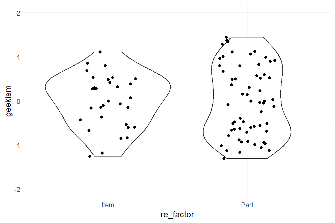
Figure 6.17: Comparing distributions of item-level and participant-level scores
Figure 6.17 shows that the 32 items of the test cover the range of very low to moderately high geekism fairly well. The upper 20 percent are not represented so well, as it seems. If we were to use the scale to discriminate between geeks and super-geeks, more strong item should be added, such as: ‘I rather express myself in a programming language, rather than natural language.’
6.8.2 Reliability
Next, we examine the reliability of the Geekism scale. Reliability is originally a CTT concept and means that the measurement error is small. For example, a reliable personality scale produces almost exactly the same score when applied to a person on different occasions. Is the Geekism score reliable? In our study we asked participants to fill out the questionnaire twice, with an experimental session in-between. If reliability of Geekism is good, the correlation of scores between sessions should be very strong.
In order to obtain the scores per session, we add Session as a factor to the model. For reliability we are interested in correlation between person scores, so it would suffice to add the Session random effect to the participant level, only. However, the same model can be used to do assess stability of item scores, too. This is rarely practiced, but as we will see, there is an interesting pattern to observe.
D_psymx_2 <-
  D_quest %>% filter(Scale == "Geek")

M_psymx_2 <-
  brm(rating ~ 0 + Session +
    (0 + Session | Part) +
    (0 + Session | Item),
  data = D_psymx_2
  )
We extract the random effects and plot test-retest scores for participants and items (Figure 6.18). The indicated line would be ideal stability for comparison.
T_ranef <-
  ranef(M_psymx_2) %>%
  select(re_factor, re_entity, Session = fixef, score = center) %>%
  pivot_wider(names_from = Session, values_from = "score")

T_ranef %>% sample_n(8)| re_factor | re_entity | Session1 | Session2 |
|---|---|---|---|
| Part | 65 | 1.012 | 0.926 |
| Part | 64 | -1.027 | -0.904 |
| Part | 8 | -1.007 | -0.912 |
| Item | Geek05 | -0.444 | -0.302 |
| Item | Geek03 | 0.765 | 0.527 |
| Item | Geek32 | -0.688 | -0.534 |
| Part | 66 | -0.955 | -0.840 |
| Part | 5 | -1.119 | -1.014 |
plot_stability <-
  function(ranef) {
    ranef %>%
      ggplot(aes(x = Session1, y = Session2)) +
      facet_grid(re_factor ~ .) +
      geom_point() +
      geom_smooth(aes(color = "observed"), se = F) +
      geom_abline(aes(
        intercept = 0, slope = 1,
        color = "ideal"
      )) +
      labs(x = "Stability")
  }

T_ranef %>% plot_stability()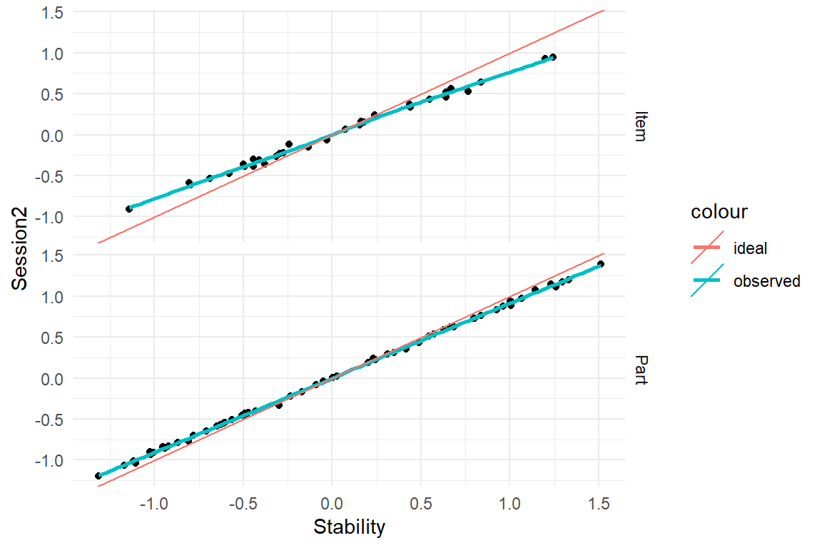
Figure 6.18: Test-retest stability for item and participant scores
The participant scores are highly correlated, indicating a very good reliability. If you measure the score of a person, you almost precisely know the result of another measure a few hours later. At least in short terms, the Geekism construct - whatever it truly is - can be measured with almost no error. Only ever so slightly is there a trend that lower scores get higher the second time and higher get lower, which could be called a trend towards the average. Perhaps, some experience during the experiment has led participants to report a more mediocre image of themselves.
In psychometric analysis it is common to assess participant-level test-retest reliability, but rarely is that done on items. This is, in fact, easy because the psychometric model contains intercept and slope random effects for items, and we can examine test-retest patterns in the same way. We see the same trend towards the average, but much stronger. In the present case, we see that this can be a mistake. Here it seems that the trend towards mediocrity does not produce a bias on the population mean, because it is bi-directional and the item and participant scores are nicely symmetric around the center of the scale. Not every test may have these properties and any asymmetric wear-off effect of items would produce more serious biases.
Another situation where item stability matters is when a person doing the test is actually learning from it. Usually, it is not desired that a test can be learned, because that means people can train for it. This is unlikely to occur in a regular math or intelligence test, but when the items are real-world tasks, like operating medical infusion pumps or driving a car, every test is an exercise and participants will learn.
The example of test-retest stability shows one more time, how useful plots are for discovering patterns in data. More formally, test-retest stability is reported as a correlation. We can produce a correlation estimate by using the standard cor command on the participant-level random effects (Table 6.25)
T_ranef %>%
  group_by(re_factor) %>%
summarize(cor = cor(Session1, Session2)) | re_factor | cor |
|---|---|
| Item | 0.997 |
| Part | 1.000 |
Unfortunately, this lacks information about the degree of certainty. The better way is to let the regression engine estimate all correlations between random factors that are on the same level (Part, Item). The regression engine brm does that by default. The following code extracts the posterior distributions of all correlations in the model (Table 6.26).
clu_cor <-
  function(model) {
    model %>%
      posterior() %>%
      filter(type == "cor") %>%
      mutate(parameter = str_remove_all(parameter, "cor_")) %>%
      group_by(parameter) %>%
      summarize(
        center = median(value),
        lower = quantile(value, .025),
        upper = quantile(value, .975)
      ) %>%
      separate(parameter,
        into = c("re_factor", "between", "and"),
        sep = "__"
      )
  }


M_psymx_2 %>%
clu_cor() | re_factor | between | and | center | lower | upper |
|---|---|---|---|---|---|
| Item | Session1 | Session2 | 0.983 | 0.913 | 0.999 |
| Part | Session1 | Session2 | 0.994 | 0.966 | 1.000 |
With random effects correlations assessing test-retest-stability is straight-forward. If test and retest random effects correlate strongly, we can be sure that the error of measurement is low and we can call it a reliable scale. Good reliability is necessary, but not sufficient to also call a scale valid.
6.8.3 Validity
Reliability doesn’t say anything about what the scale actually measures. In psychometric studies, validity of a scale is routinely evaluated by comparing the scores to external criteria. In a perfect world, it would be assessed how scores are related to relevant real-world behavior, such as:
- Are high-Geek persons more enthusiastic to learn a programming language?
- Do high-Geek persons perform better in computer jobs?
- Are high-Geek persons more likely to buy robot toys for their offsprings?
In the real world, researchers in the field of personality are often content with relating a new rating scales to another, already validated personality scale. In the Hugme study, participants were also asked to rate themselves on the Need-for-Cognition scale (NCS). In very brief NCS measures how much a person enjoys intellectual puzzles. Since computers are intellectual puzzles, sometimes in a good way, often not, we thought that high-Geek persons must also score high on NCS. At the same time, a very strong correlation between Geek and NCS would indicate that the two scales render the same property, which would make one of them redundant, probably the newcomer. The following model estimates the person scores per scale and we can extract the correlations (Table 6.27).
M_psymx_3 <-
  D_quest %>%
  brm(rating ~ 0 + Scale + (0 + Scale | Part), data = .)
M_psymx_3 %>%
clu_cor() | re_factor | between | and | center | lower | upper |
|---|---|---|---|---|---|
| Part | ScaleGeek | ScaleNCS | 0.371 | 0.098 | 0.586 |
Table 6.27 shows a weakly positive association between Geek and NCS, just as was hoped for. The two constructs are related, but not quite the same.
6.8.4 Towards Design-o-metrix
Psychometrics, as it was introduced above, deals with comparing human individuals. In Design Research, this may be of interest sometimes, but the real stake is to compare designs. As we will see in this section, psychometric concepts can well be transferred to design-o-metric problems. However, there is one twist, which has up til now been overlooked in most of Design Research: in design-o-metric studies the target population is designs, not humans. In a typical psychometric study, measurements are an encounter of humans with items, with the ultimate goal of measuring humans. A design-o-metric measurement is the encounter of three populations, humans, items and, ultimately, designs. Classic psychometric tools use a 2-dimensional matrix as input and cannot deal with a third dimension. Here it comes in very handy, that multi-level models use the long format, where more dimension can be added at will. All we have to do, is crossing in another non-human population 6.5.
We revisit the Uncanny Valley data set (5.5 and 6.4). The experiment used eight items from the Eeriness scale (Ho and MacDorman 2017) to ask the judgment of participants on 82 stimuli showing robot faces. In one of our experiments (RK_1), participants simply rated all robots face in three separate session. Since we are only interested in a design-o-metric analysis regarding the Eeriness scale, not the Uncanny Valley curve, we omit the human-likeness score (Table 6.28).
attach(Uncanny)UV_dsgmx <-
RK_1 %>%
select(Part, Item, Design = Stimulus, Session, response) %>%
as_tbl_obs()
UV_dsgmx| Obs | Part | Item | Design | Session | response |
|---|---|---|---|---|---|
| 1242 | p1_05 | nE2 | 3 | 1 | -0.967 |
| 4566 | p2_03 | nE6 | 71 | 3 | -0.740 |
| 4589 | p2_03 | nE5 | 8 | 3 | -0.258 |
| 5252 | p2_06 | nE4 | 72 | 1 | -0.352 |
| 5362 | p2_06 | nE2 | 73 | 2 | -0.705 |
| 6506 | p2_10 | nE2 | 46 | 2 | -0.670 |
| 7035 | p2_12 | nE3 | 14 | 2 | -0.567 |
| 7345 | p2_13 | nE1 | 69 | 2 | -0.688 |
With this data we seem to be standing on familiar psychometric grounds: Persons encounter items and we have three measures over time. We can calculate test-retest stability of items and persons using a multi-level model. Voila! Here are your correlations, person and item stability - with credibility limits. But, wait a second! What is being measured here? Persons? No, robot faces. The original question was, how human-likeness of robot faces is related to perceived eeriness of robot faces and the Eeriness scale intended purpose is the comparison of designs, not persons. For example, it could be used by robot designers to check that a design does not trigger undesirable emotional responses. Without knowing the human-likeness scores, robot faces become just a naked population of designs 6.5.
Measures in the Uncanny experiment are an encounter of three samples: Part, Item and Design, and designs is what we ultimately want to compare. That means we need a model that produces design-level scores. For the user of multi-level models that just means adding a Design random effect to the psychometric model (Part, Item). Models, where a design random factor sits on top of a psychometric model, I call design-o-metric models. The most basic design-o-metric model is a three-way cross-classified, intercept-only model, from which design scores can be extracted. By extending the test-retest psychometric model M_psymx_2, we can estimate design-o-metric test-retest stability. We only have to add the Design random factor to the model and extract the correlations, like in the psychometric applications.
M_dsgmx_1 <-
  brm(response ~ 0 + Session +
    (0 + Session | Part) +
    (0 + Session | Item) +
    (0 + Session | Design),
  data = UV_dsgmx
  )
M_dsgmx_1 %>%
clu_cor() | re_factor | between | and | center | lower | upper |
|---|---|---|---|---|---|
| Design | Session1 | Session2 | 0.987 | 0.945 | 0.999 |
| Design | Session1 | Session3 | 0.987 | 0.946 | 0.999 |
| Design | Session2 | Session3 | 0.991 | 0.961 | 0.999 |
| Item | Session1 | Session2 | 0.849 | 0.228 | 0.989 |
| Item | Session1 | Session3 | 0.702 | -0.066 | 0.958 |
| Item | Session2 | Session3 | 0.841 | 0.170 | 0.988 |
| Part | Session1 | Session2 | 0.816 | 0.557 | 0.950 |
| Part | Session1 | Session3 | 0.686 | 0.377 | 0.869 |
| Part | Session2 | Session3 | 0.815 | 0.570 | 0.930 |
Like in the psychometric situation, we extract the correlations (6.29). Since we have three sessions, we even get three stability scores. In addition, the design-o-metric model provides test-retest correlations for all three levels. The test-retest stability for designs is very reassuring. Ratings on the Eeriness scale are highly reproducible and the error will be very small. To a lesser, but still sufficient degree are person and item scores stable.
But, what does the person score (and its stability) actually mean? It describes the tendency of a person to give high ratings on Eeriness. Should a researcher want to assess how sensitive a person is to the Uncanny Valley effect, the Eeriness scale is also reliable for measuring persons. Many scales in design research lend themselves to be looked at from a design-o-metric and psychometric perspective. For example, a hypothetical scale to measure comfort of sitting can be used to evaluate seats, but can also be used to measure how comfortable a person is with sitting.
No seat fits every person, or put differently: the comfort of a seat depends on the person sitting in it. This points us at one of many possible extensions to carry out deeper design-o-metric analysis. If the difficulty of an item in a psychometric test depends on who is being tested, this is called differential item functioning. For example, the large international student evaluations PISA and TIMMS routinely check their test items for cultural differences. The aim is to formulate test questions in such a way that they are equally comprehensible with all cultural backgrounds. This is a desirable property for design-o-metric scales, too. In a multi-level design-o-metric model, this could be incorporated as an interaction effect between cultural background and item-level coefficients.
That all being said about design-o-metric models, my observation is that practically all published rating scales in design research have been validated under a psychometric perspective, rather than a design-o-metric. This is a mistake! If the purpose of the scale is to compare designs, the scale’s reliability and validity must examined on the design level.
In many cases, a purportedly design-o-metric study has been conducted on a sample of participants and a sample of items, but only a single or a few designs. Isn’t it obvious that a scale’s capability to rank designs must be assessed on a sample of designs. This mindlessness in transfering psychometric concepts to design research is worrying and I call this the psychometric fallacy.
6.9 Further readings
- In psychometric models the population level is of lesser interest. One could build a single-level model, using fixed-effects factors for participants and items. (Gelman, Hill, and Yajima 2012) show that random-effects models are superior, because they allow multiple pairwise comparisons, which is problematic with fixed effects. For psychometric situations, comparison of individuals is essential.
- An introduction to planned missing data designs, as we used it in cases Egan and Uncanny, is given by (Graham et al. 2006).
- Multi-level models for psycholinguistic studies have been used by (Baayen, Davidson, and Bates 2008).
- In (Schmettow and Sommer 2016), we evaluated whether we can predict by the method of card sorting, how quickly users find a specific information on a website. A multi-level model showed that this is not so. This serves as an example, that you can prove the (practical) absence of effects with New Statistics, and publish.
- (Ho and MacDorman 2017) is one of many examples of falling for the psychometric fallacy.